When can a CCD constrain the metallicity of hot halo gas?
A fakeit study built on the XMM-Newton EPIC MOS observation of M104 (NGC 4594, ObsID 0900170101): absolute metallicity and the O/Fe ratio as a function of plasma temperature, surface brightness and exposure, with the real sky background, soft-proton and instrumental-line model of that field.
2026-09-24, revised 2026-09-25XMM-Newton EPIC MOS1+MOS2Sherpa 4.18 / XSPEC 12.14 apec & vapecsingle-realization Δχ² profiles中文
Result in one paragraph. For a ~0.7 keV halo at the surface brightness of M104's inner halo (6.6–16.5 kpc, 1× F₀) the CCD spectrum gives only a lower bound on the metallicity unless the true Z is low: with the soft protons free, six times the current exposure (≈400 ks clean per camera) constrains Zin to 0.14–0.52 if the truth is 0.3, but only to Zin > 0.34 if the truth is 1, and the outer annulus (16.5–30 kpc, 0.3× F₀) stays open-ended in both cases. Simulating each annulus with its own responses and background, the inner annulus (79 arcmin² effective, 1× F₀) needs 1000 ks of clean exposure for a factor-of-3 constraint if the true Z is 0.3 (3000 ks for a factor of 2), 10 Ms if it is 1, and is never bounded from above if it is 3; the outer annulus (212 arcmin² effective, 0.3× F₀) needs 1000 ks for a true Z of 0.1, 3000 ks for 0.3, and never closes for Z ≥ 1 while the soft protons are free. A known soft-proton shape cuts these by a factor of 3–10. Absolute Z is measured to a factor of 2 in 100 ks only for kT ≳ 1.5 keV at ≥3× F₀, or for kT ≥ 1 keV at 10× F₀, and a metal-rich plasma (Z ≥ 1) is the hardest case at every temperature because its continuum is faint. The line-to-line O/Fe ratio (vapec) is the complementary observable: at 1× F₀ and 100 ks solar O/Fe is bounded to within a factor of 3 for kT ≤ 0.7 keV, and at ≥3× F₀ to within a factor of 2, but an iron-rich ratio (O/Fe ≤ 0.3) yields only upper limits below 3× F₀. Longer exposure does help once the continuum is detectable (kT ≥ 1 keV, or a low true Z); for a 0.7 keV, metal-rich halo it does not within any realistic programme.
1. Setup
Data products and geometry
- ObsID 0900170101 (XART-ATOMS central field), MOS1 and MOS2, ESAS products with point sources masked. Two full annuli: R2–5′ (6.6–16.5 kpc; 36.6 and 42.3 arcmin² on MOS1/MOS2) and R5–9′ (16.5–30 kpc; 81.8 and 129.8 arcmin²). Clean exposure 65.8 / 65.2 ks per camera. Each annulus has its own ARF, RMF and quiescent-particle-background (QPB) spectrum.
- Extraction sky area. The generalised grids (Sections 3–5) use the R2–5′ geometry only: 36.6 arcmin² on MOS1 and 42.3 arcmin² on MOS2 (79 arcmin² in total, the two cameras differ because of masked point sources and CCD gaps). All count numbers on this page refer to that area. At fixed surface brightness the source counts scale linearly with area, so a region of area A behaves like this one at a surface brightness of (A / 79 arcmin²) × F; e.g. a 20 arcmin² region at 4× F₀ has the same source counts as this geometry at 1× F₀, while the sky, soft-proton and QPB counts scale with area as well, so the source fraction per band is unchanged. Reading the maps by total source counts (listed under each table) is the safest way to transfer them to another region size.
- Distance scale 3.3 kpc / arcmin as in the XART-ATOMS analysis. pn is not included (no per-annulus pn products); see caveats.
Sky background, soft protons, instrumental lines
All non-source components take the best-fit values of the production analysis of this field, in which the sky components were fixed from the dedicated offset field (ObsID 0900170701):
| Component | Model | Value (per arcmin²) | In the fit |
|---|---|---|---|
| Local Hot Bubble | apec, kT = 0.083 keV, Z = 1 | norm 3.41 × 10⁻⁶ | fixed |
| Milky Way halo | apec, kT = 0.177 keV, Z = 0.3, absorbed | norm 4.53 × 10⁻⁶ | fixed |
| Cosmic X-ray background | pegpwrlw, Γ = 1.46, 0.5–2 keV, absorbed | 1.05 × 10⁻¹⁵ erg cm⁻² s⁻¹ | fixed (±10% variants tested) |
| Absorption | phabs | NH = 3 × 10²⁰ cm⁻² | fixed |
| Soft protons | powerlaw through RMF only (unit ARF) | Γ ≈ 1.2–1.3; norm ≈ 3.0 × 10⁻⁴ (R2–5) and 1.5 × 10⁻⁴ (R5–9) ct s⁻¹ keV⁻¹ at 1 keV, MOS1; MOS2 × 0.7 | index and norm free, per camera |
| Instrumental lines | Gaussians at 1.49, 1.75 keV (Al K, Si K) and 1.28 keV | from the production fit | norms free, per camera |
Source and sky components are folded through ARF × RMF × exposure; the soft-proton component through RMF × exposure with a unit ARF, so its normalisation is a count rate, not a flux. The truth model reproduces the observed QPB-subtracted count rates band by band to 1–3% on MOS1 and 5–15% on MOS2 (Figure 4).
Source and brightness scale
- Source: absorbed
apec(orvapec) at redshift 0.003416. For the M104 case kT = 0.72 / 0.71 keV (R2–5 / R5–9). - F₀ = 2.68 × 10⁻¹⁵ erg cm⁻² s⁻¹ arcmin⁻²: the absorbed 0.5–2 keV surface brightness of M104's R2–5′ annulus. The grids use 0.3×, 1×, 3× and 10× F₀. For reference, the same scale in M104 itself: 0.5–1′ ≈ 10× F₀, 1–2′ ≈ 3.7× F₀, 2–4′ ≈ 1× F₀ (from the published annular fluxes), 5–9′ ≈ 0.3× F₀.
- Two normalisation conventions. In the M104 two-zone case (Section 2) the source normalisation is rescaled for every trial Z so that the 0.7–1.0 keV (Fe-L) source counts stay equal to what is observed: the known quantity is the Fe-L flux, the unknown is Z. In the grids (Sections 3–6) the normalisation is instead set so that the absorbed 0.5–2 keV surface brightness equals the stated multiple of F₀ for every true Z. Because Fe-L dominates the 0.5–2 keV band of a 0.7 keV plasma the two conventions are close but not identical: at kT = 0.7 keV, 1× F₀ and 100 ks the Fe-L source counts rise from 1650 at Ztrue = 0.1 to 2200 at Ztrue = 3.
Simulation and fitting contract
- Fake source spectrum = Poisson(model + F × QPB); fake QPB = Poisson(F × QPB); exposure = F × 65.8 ks. F = 1 is the current data; F = 4 / 5 / 6 ≈ +300 / 400 / 500 ks raw at 75% cleaning efficiency; the grids use 100 ks and 300 ks directly.
- Fit: QPB subtracted, 0.4–3.2 keV (M104 case) or 0.4–7 keV (grids), ≥25 counts per bin,
chi2gehrels,levmar. Free: kT, norm, Z (or Fe and O), soft-proton index and norm per camera, instrumental-line norms per camera. - Δχ² profile: Z (or O/Fe) fixed on a grid 0.05–5 (0.1–5 for O/Fe); everything else refitted at every grid point. Intervals are read at Δχ² = 1 (68%) and 4 (95%) after interpolation in log Z. "Within a factor of 2" means both 95% bounds are inside [truth/2, 2 × truth]; "within a factor of 3" means both are inside [truth/3, 3 × truth]. Section 5 reports both criteria as a function of the true value.
2. The M104 case: a lower bound on Zin, and an upper bound only if the halo is metal-poor
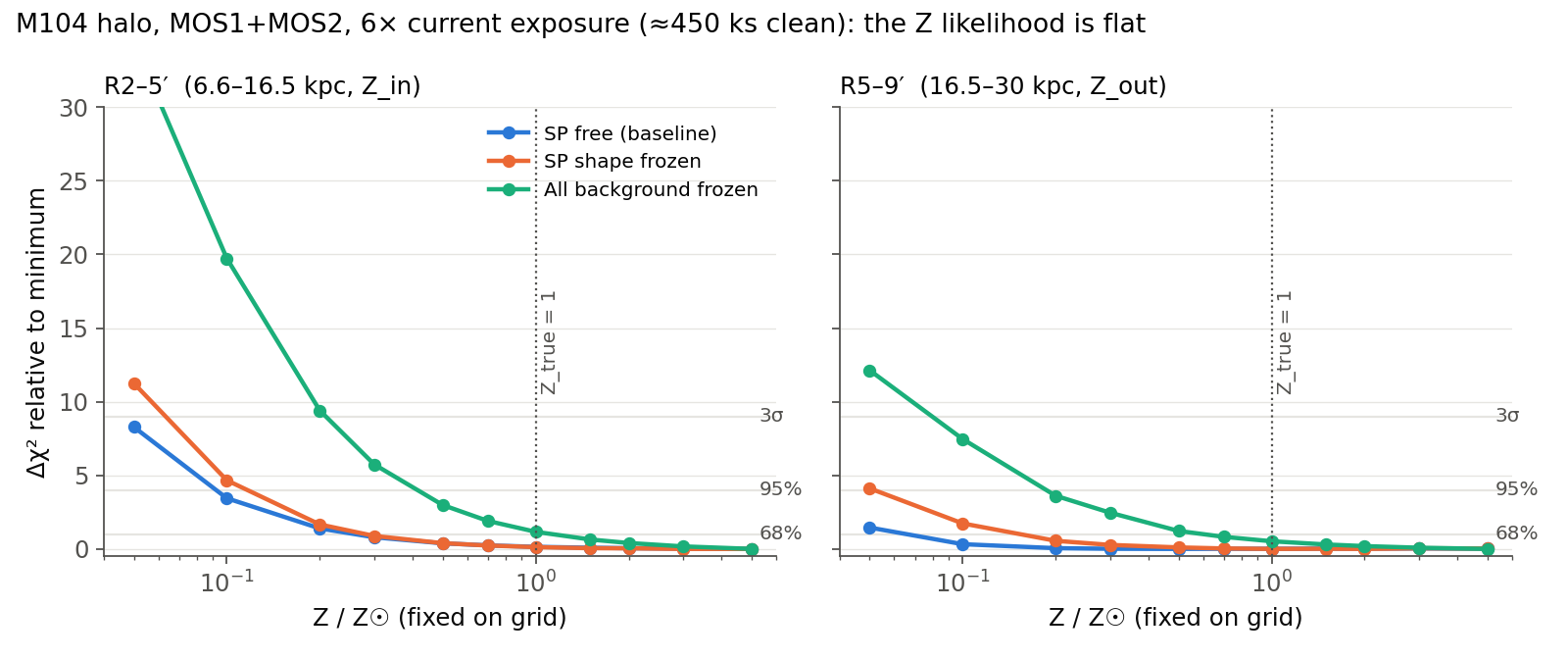
| Contract | Case | R2–5′ (Zin), 95% | R5–9′ (Zout), 95% |
|---|---|---|---|
| SP free | F = 6, Ztrue = 1 | 0.34–5+ (lower bound only; best fit at 2) | 0.30–5+ (lower bound only) |
| SP free | F = 6, Ztrue = 0.3 | 0.14–0.53 (68%: 0.18–0.31) | 0.23–5+ (lower bound only) |
| SP free | F = 1, Ztrue = 0.3 (current data) | <0.05–4.3: unconstrained | unconstrained |
| SP shape frozen | F = 6, Ztrue = 1 | 0.29–5+ (68%: 0.44–1.5) | 0.17–5+ |
| All background frozen | F = 6, Ztrue = 1 | 0.53–3.7 (68%: 0.69–1.5) | 0.33–5+ (68%: 0.48–1.8) |
| All background frozen | F = 6, Ztrue = 0.3 | 0.30–0.69 (68%: 0.42–0.54) | 0.26–2.8 (68%: 0.39–0.87) |
Three things follow. First, the current 66 ks are uninformative about Z in either annulus, at any true value. Second, six times the exposure gives a robust lower bound on Zin (Z > 0.3 at 95% if the halo is solar) but an upper bound only if the halo is metal-poor: a true Zin of 0.3 is recovered to within a factor of 2 with the soft protons free, whereas a solar or super-solar halo runs off the top of the grid. Third, knowing the background does not change the picture qualitatively: with every nuisance component frozen at truth, Zin = 1 is bounded only to 0.5–3.7, and Zout stays open-ended for a solar halo. The outer annulus (16.5–30 kpc) is not measurable in any contract unless its metallicity is low. A Monte-Carlo grid of eight full two-zone fits per configuration (F = 1, 4, 6; Ztrue = 0.3, 1, 2; CXB ±10%; a 30% cool-phase injection; every realization generated from the same truth) says the same thing in point estimates: for Ztrue = 0.3 the recovered Zin is 0.25 (16–84%: 0.21–0.43) at F = 6 and 0.37 (0.27–0.47) at F = 4, with Zout 0.34 (0.23–0.95) and 0.23 (0.11–1.5); for Ztrue = 1 at F = 6 Zin is 0.92 (0.57–1.5) while Zout piles up at the grid boundary of 5 (0.90–5), and at F = 4 Zin scatters over 0.67–5; for Ztrue = 2 the medians are 1.9 (0.8–3.7) and 2.0 (0.7–5). kT is recovered to ±0.005–0.025 keV throughout; a 30% cool-phase injection fitted with one temperature biases kTin to 0.67 keV and Zin to 0.74 (0.40–1.1), and a ±10% CXB error spreads Zin over 0.8–3.3. Data: summary.csv.
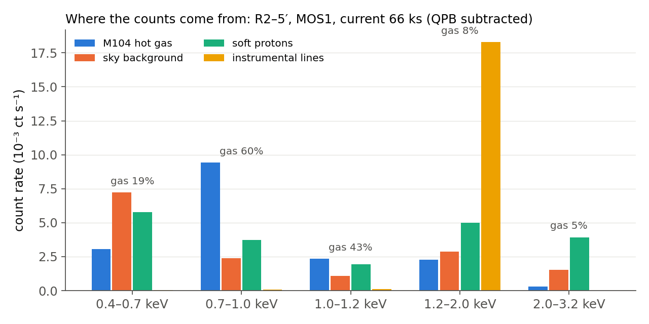
| Band (keV) | data − QPB | model total | M104 gas | sky | soft protons | lines | gas fraction |
|---|---|---|---|---|---|---|---|
| 0.4–0.7 | 15.2 | 16.1 | 3.06 | 7.24 | 5.78 | 0.05 | 19% |
| 0.7–1.0 | 15.2 | 15.6 | 9.42 | 2.40 | 3.73 | 0.07 | 60% |
| 1.0–1.2 | 5.6 | 5.5 | 2.36 | 1.07 | 1.93 | 0.11 | 43% |
| 1.2–2.0 | 28.4 | 28.4 | 2.29 | 2.87 | 4.99 | 18.28 | 8% |
| 2.0–3.2 | 5.6 | 5.8 | 0.30 | 1.53 | 3.93 | 0.02 | 5% |
Count rates in 10⁻³ ct s⁻¹, R2–5′, MOS1, QPB subtracted; all components in the same units.
3. Absolute metallicity: temperature × surface brightness × exposure (true Z = 0.5)
Everything in this section assumes a true metallicity of Z = 0.5 Z☉, a single realization per cell, MOS1+MOS2, 79 arcmin², M104 sky background, soft protons free, 0.4–7 keV. Section 5 repeats the 100 ks grid for true Z = 0.1, 0.3, 1 and 3, because the answer depends on the truth: at fixed 0.5–2 keV surface brightness a lower true Z means a brighter continuum and an easier upper bound.
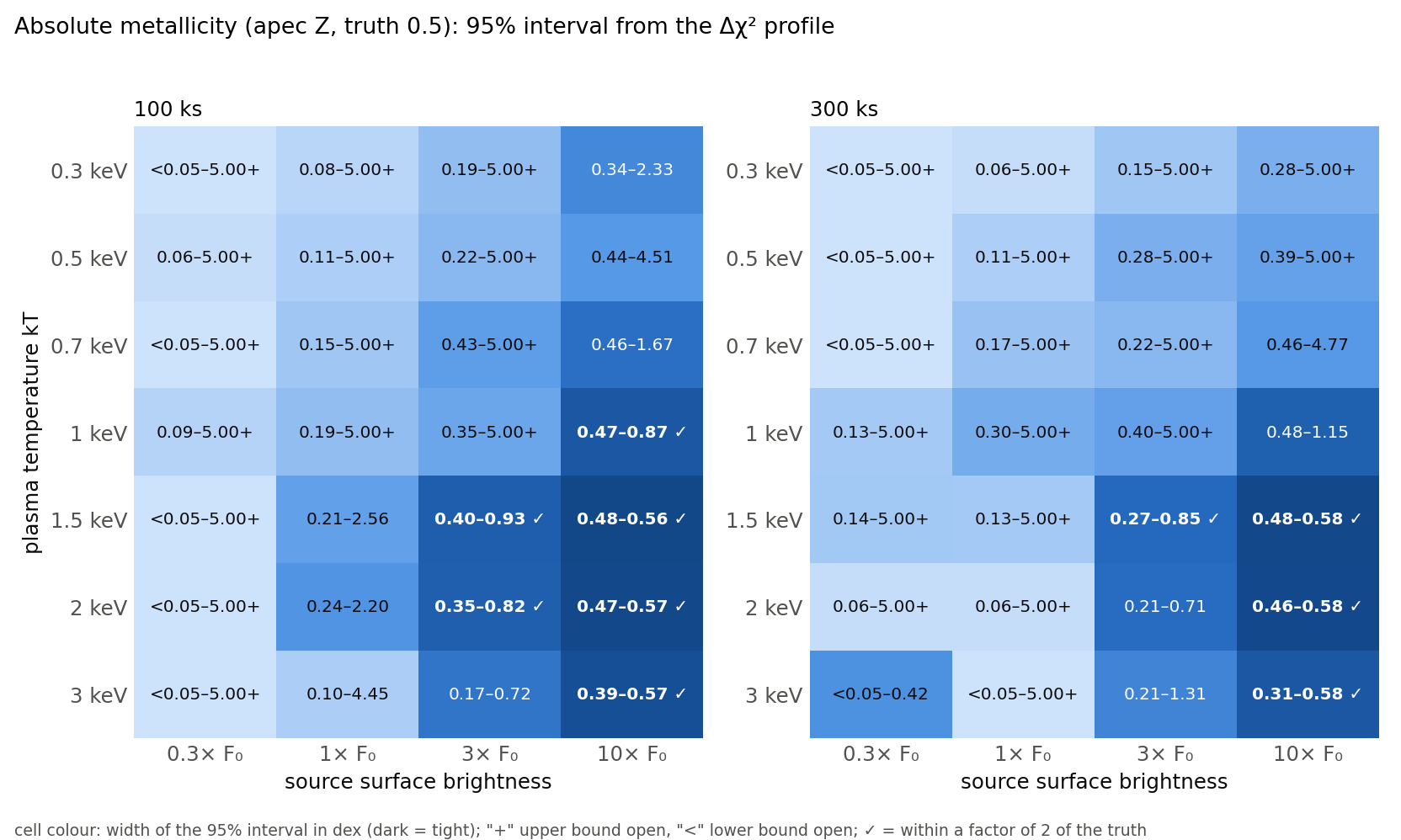
100 ks — true Z = 0.5, 95% interval on Z
| kT | 0.3× F₀ | 1× F₀ | 3× F₀ | 10× F₀ |
|---|---|---|---|---|
| 0.3 keV | unconstrained | 0.09–5.00+ | 0.20–5.00+ | 0.37–0.95 |
| 0.5 keV | 0.09–5.00+ | 0.22–5.00+ | 0.34–5.00+ | 0.47–2.53 |
| 0.7 keV | unconstrained | 0.21–5.00+ | 0.33–5.00+ | 0.47–1.18 |
| 1 keV | 0.15–5.00+ | 0.28–5.00+ | 0.41–2.65 | 0.49–0.82 |
| 1.5 keV | 0.08–5.00+ | 0.24–2.06 | 0.42–0.72 | 0.49–0.51 |
| 2 keV | unconstrained | 0.22–1.40 | 0.36–0.65 | 0.49–0.53 |
| 3 keV | unconstrained | 0.22–2.74 | 0.22–0.76 | 0.43–0.54 |
300 ks — true Z = 0.5, 95% interval on Z
| kT | 0.3× F₀ | 1× F₀ | 3× F₀ | 10× F₀ |
|---|---|---|---|---|
| 0.3 keV | 0.07–5.00+ | 0.23–5.00+ | 0.37–5.00+ | 0.47–0.78 |
| 0.5 keV | 0.06–5.00+ | 0.18–5.00+ | 0.30–1.28 | 0.48–0.72 |
| 0.7 keV | 0.07–5.00+ | 0.19–5.00+ | 0.36–1.22 | 0.49–0.65 |
| 1 keV | 0.12–5.00+ | 0.27–1.85 | 0.44–0.74 | 0.50–0.57 |
| 1.5 keV | 0.14–4.89 | 0.36–0.80 | 0.48–0.56 | 0.50–0.51 |
| 2 keV | 0.08–1.00 | 0.27–0.66 | 0.47–0.55 | 0.50–0.50 |
| 3 keV | <0.05–4.67 | 0.19–1.08 | 0.42–0.66 | 0.49–0.51 |
Green = within a factor of 2 at 95%, blue = within a factor of 3, grey = a bound is open. Source counts for reference (both cameras, 100 ks, 1× F₀): 1500–2000 in the Fe-L band for kT ≤ 1 keV, 700–850 for kT ≥ 1.5 keV; 3200–4600 in 0.4–7 keV. Full table with 68% intervals and best-fit values: summary_ccdZ.csv; per-cell profiles in data/profiles_Z/.
Reading the map
- Temperature is the first-order control. For kT ≤ 1 keV at 100 ks, Z has only a lower bound unless the surface brightness reaches 10× F₀ (and even there 0.5 keV gas gives 0.47–2.5). The profile falls monotonically with Z: the fit prefers to give the continuum to the free soft-proton component and make the source pure line emission, so the minimum sits at the upper boundary.
- For kT ≥ 1.5 keV the bremsstrahlung extends to 2–7 keV and Fe K appears: at 3× F₀ 100 ks is enough for a factor-of-2 constraint, and at 1× F₀ 300 ks is (0.36–0.80 at 1.5 keV, 0.27–0.66 at 2 keV). kT = 1 keV is transitional: factor 2 at 10× F₀ in 100 ks or at 3× F₀ in 300 ks.
- Exposure helps where a continuum is detectable, and not otherwise. Going from 100 to 300 ks moves the (1× F₀, kT ≥ 1.5 keV) and (3× F₀, kT = 0.5–1 keV) cells into the constrained region, but leaves every kT ≤ 0.7 keV cell at ≤3× F₀ open-ended. Section 6 follows the 0.7 keV case to much larger area × exposure products.
- M104's inner halo sits in the (0.7 keV, 1× F₀) cell: 0.21–5+ at 100 ks and 0.19–5+ at 300 ks. Its outer halo (0.3× F₀) is unconstrained at every temperature except 2 keV at 300 ks.
- Single realizations: several 300 ks cells look no better than their 100 ks counterparts (e.g. 3 keV at 1× F₀), which is realization scatter of roughly ±50% in the interval bounds, not a trend.
4. Line-to-line: the O/Fe ratio with vapec (true O/Fe = 1.0)
Everything in this section assumes a true O/Fe of 1.0 (Fe = O = 0.5 Z☉), same geometry, background and exposure conventions as Section 3. Section 5 repeats the 100 ks grid for true O/Fe = 0.1, 0.3 and 3.
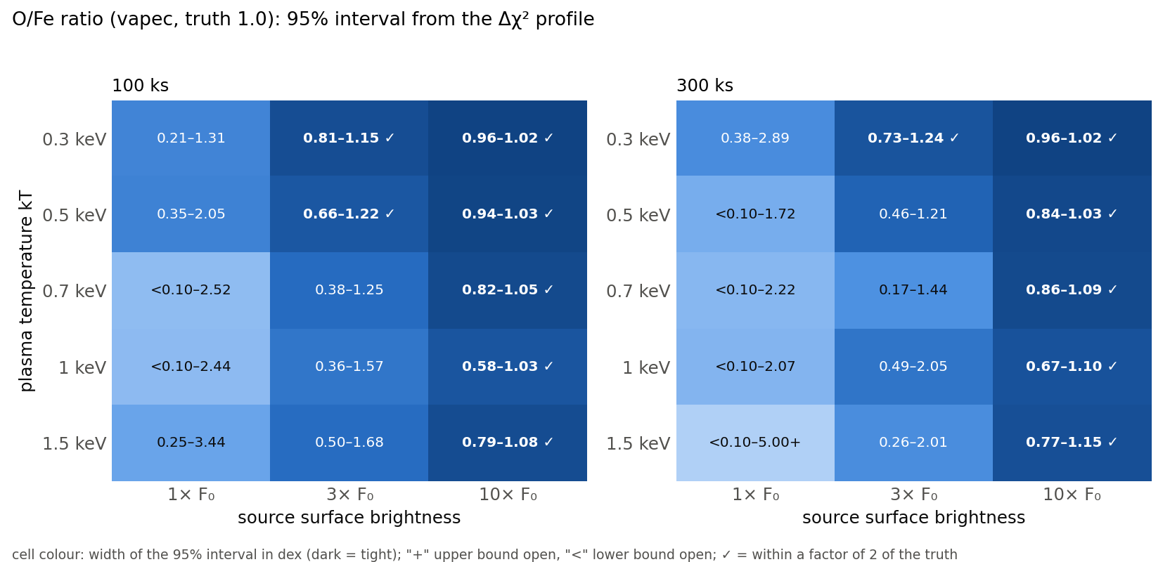
vapec: Fe free (Ni tied), O free (C, N, Ne, Mg, Al, Si, S, Ar, Ca tied to O), kT and norm free, soft protons and lines free. The foreground O VII / O VIII of the Local Hot Bubble and Milky Way halo are fixed at their true values (an optimistic assumption, see caveats).100 ks — true O/Fe = 1.0, 95% interval on O/Fe
| kT | 1× F₀ | 3× F₀ | 10× F₀ |
|---|---|---|---|
| 0.3 keV | 0.45–1.37 | 0.83–1.07 | 0.98–1.01 |
| 0.5 keV | 0.35–1.48 | 0.84–1.14 | 0.95–1.01 |
| 0.7 keV | 0.44–2.17 | 0.57–1.21 | 0.90–1.03 |
| 1 keV | 0.09–2.47 | 0.45–1.27 | 0.87–1.05 |
| 1.5 keV | 0.51–3.03 | 0.57–1.34 | 0.70–1.03 |
300 ks — true O/Fe = 1.0, 95% interval on O/Fe
| kT | 1× F₀ | 3× F₀ | 10× F₀ |
|---|---|---|---|
| 0.3 keV | 0.85–1.21 | 0.97–1.02 | 0.99–1.00 |
| 0.5 keV | 0.60–1.25 | 0.92–1.03 | 0.99–1.00 |
| 0.7 keV | 0.19–1.25 | 0.79–1.05 | 0.97–1.01 |
| 1 keV | 0.07–1.34 | 0.54–1.03 | 0.97–1.00 |
| 1.5 keV | <0.03–1.18 | 0.84–1.11 | 0.96–1.00 |
Source counts (both cameras, 100 ks, 1× F₀): 300–1100 in the O band (0.5–0.7 keV), 850–2040 in the Fe-L band. Full table: summary_OFe.csv; per-cell profiles in data/profiles_OFe/.
Reading the map
- O/Fe is a much better CCD observable than absolute Z because both ends are lines and neither depends on the soft-proton-dominated continuum. It is constrained exactly where absolute Z fails: cool gas (kT ≤ 0.7 keV) reaches ±10–30% at 3× F₀ in 100 ks, and every kT ≤ 1.5 keV reaches ±3–15% at 10× F₀. The two maps are nearly complementary: absolute Z wants hot gas, O/Fe wants cool gas with strong O VIII.
- For M104's inner halo (0.7 keV, 1× F₀) solar O/Fe is bounded to 0.44–2.2 in 100 ks (within a factor of 3) and 0.19–1.25 in 300 ks: it can exclude strongly α-enhanced gas, and at 300 ks starts to separate a Type Ia signature (O/Fe ≈ 0.3) from solar, but only if the foreground oxygen lines are known (see caveats).
- M104's bulge (r < 2′, 4–10× F₀) is in the constrained region: O/Fe to ±10–20% in 100 ks, consistent with the ±0.5 obtained from 200 ks of Chandra within 5′ in the literature. The absolute Fe stays unconstrained in most cells (best-fit Fe at the boundary).
5. Dependence on the true value: where is the constraint within a factor of 3, or 2?
Sections 3–4 fix the truth at Z = 0.5 and O/Fe = 1. Because every trial spectrum is normalised to the same absorbed 0.5–2 keV surface brightness, a higher true Z means a fainter continuum (the lines take a larger share of a fixed broadband flux; for a 0.7 keV plasma the Fe-L counts rise only from 1650 to 2200 between Z = 0.1 and 3, so this is close to, but not the same as, the fixed-Fe-L convention of the M104 case in Section 2): upper bounds get harder and lower bounds easier as the truth rises, and the reverse for a low truth. The grids below repeat the 100 ks profiles for Ztrue = 0.1, 0.3, 1 and 3 (with the Z = 0.5 grid from Section 3) and O/Fetrue = 0.1, 0.3 and 3 (with the O/Fe = 1 grid from Section 4). Extraction area 79 arcmin² (36.6 + 42.3 arcmin², MOS1 + MOS2), M104 sky background, soft protons free. The Z profile grid runs 0.05–5 for Ztrue ≤ 1 and 0.05–20 for Ztrue = 3 (XSPEC apec caps its abundance at 5, so the extended runs use vapec with every metal tied to Fe, which is the same model); the O/Fe grid runs 0.1–5 for O/Fetrue = 1 and 0.03–10 for the other truths. An open bound ("+" or "<") therefore means the profile is still within Δχ² = 4 of its minimum at the edge of the scanned range. Two criteria are marked: ✓✓ both 95% bounds within [truth/2, 2 × truth] and ✓ both within [truth/3, 3 × truth].
Absolute metallicity
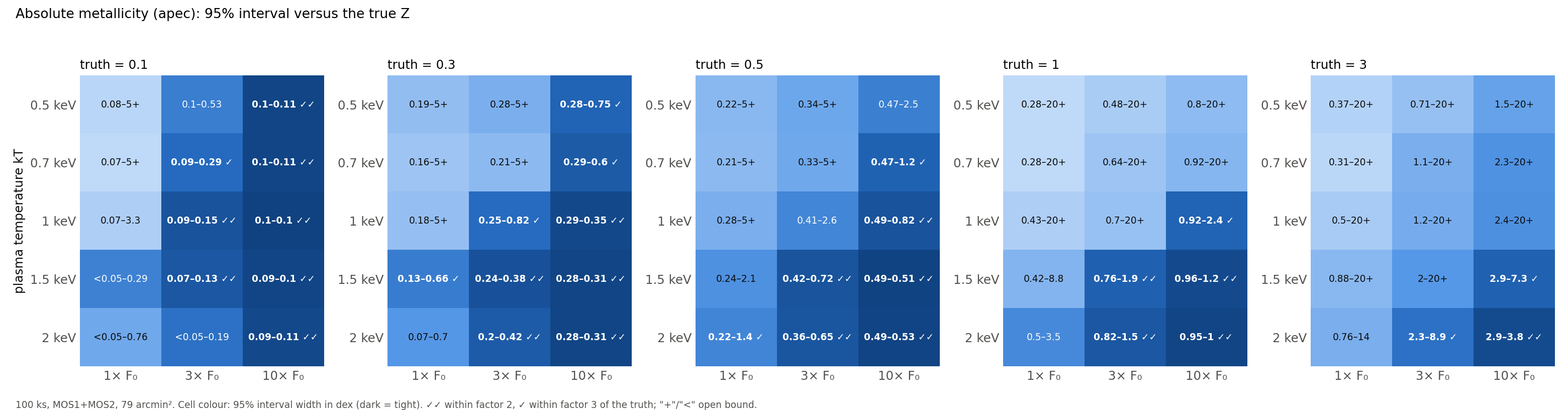
truth = 0.1
| kT | 1× F₀ | 3× F₀ | 10× F₀ |
|---|---|---|---|
| 0.5 keV | 0.08–5.00+ | 0.10–0.53 | 0.10–0.11 |
| 0.7 keV | 0.07–5.00+ | 0.09–0.29 | 0.10–0.11 |
| 1 keV | 0.07–3.26 | 0.09–0.15 | 0.10–0.10 |
| 1.5 keV | <0.05–0.29 | 0.07–0.13 | 0.09–0.10 |
| 2 keV | <0.05–0.76 | <0.05–0.19 | 0.09–0.11 |
truth = 0.3
| kT | 1× F₀ | 3× F₀ | 10× F₀ |
|---|---|---|---|
| 0.5 keV | 0.19–5.00+ | 0.28–5.00+ | 0.28–0.75 |
| 0.7 keV | 0.16–5.00+ | 0.21–5.00+ | 0.29–0.60 |
| 1 keV | 0.18–5.00+ | 0.25–0.82 | 0.29–0.35 |
| 1.5 keV | 0.13–0.66 | 0.24–0.38 | 0.28–0.31 |
| 2 keV | 0.07–0.70 | 0.20–0.42 | 0.28–0.31 |
truth = 0.5
| kT | 1× F₀ | 3× F₀ | 10× F₀ |
|---|---|---|---|
| 0.5 keV | 0.22–5.00+ | 0.34–5.00+ | 0.47–2.53 |
| 0.7 keV | 0.21–5.00+ | 0.33–5.00+ | 0.47–1.18 |
| 1 keV | 0.28–5.00+ | 0.41–2.65 | 0.49–0.82 |
| 1.5 keV | 0.24–2.06 | 0.42–0.72 | 0.49–0.51 |
| 2 keV | 0.22–1.40 | 0.36–0.65 | 0.49–0.53 |
truth = 1
| kT | 1× F₀ | 3× F₀ | 10× F₀ |
|---|---|---|---|
| 0.5 keV | 0.28–20.00+ | 0.48–20.00+ | 0.80–20.00+ |
| 0.7 keV | 0.28–20.00+ | 0.64–20.00+ | 0.92–20.00+ |
| 1 keV | 0.43–20.00+ | 0.70–20.00+ | 0.92–2.41 |
| 1.5 keV | 0.42–8.76 | 0.76–1.86 | 0.96–1.22 |
| 2 keV | 0.50–3.50 | 0.82–1.53 | 0.95–1.04 |
truth = 3
| kT | 1× F₀ | 3× F₀ | 10× F₀ |
|---|---|---|---|
| 0.5 keV | 0.37–20.00+ | 0.71–20.00+ | 1.53–20.00+ |
| 0.7 keV | 0.31–20.00+ | 1.12–20.00+ | 2.27–20.00+ |
| 1 keV | 0.50–20.00+ | 1.17–20.00+ | 2.41–20.00+ |
| 1.5 keV | 0.88–20.00+ | 2.00–20.00+ | 2.93–7.31 |
| 2 keV | 0.76–13.74 | 2.34–8.89 | 2.88–3.78 |
Cells that satisfy each criterion, 100 ks:
| truth | cells within a factor of 3 (95%) | cells within a factor of 2 (95%) |
|---|---|---|
| Z = 0.1 | 3× F₀: kT = 0.7, 1, 1.5; 10× F₀: kT = 0.5, 0.7, 1, 1.5, 2 | 3× F₀: kT = 1, 1.5; 10× F₀: kT = 0.5, 0.7, 1, 1.5, 2 |
| Z = 0.3 | 1× F₀: kT = 1.5; 3× F₀: kT = 1, 1.5, 2; 10× F₀: kT = 0.5, 0.7, 1, 1.5, 2 | 3× F₀: kT = 1.5, 2; 10× F₀: kT = 1, 1.5, 2 |
| Z = 0.5 | 1× F₀: kT = 2; 3× F₀: kT = 1.5, 2; 10× F₀: kT = 0.7, 1, 1.5, 2 | 3× F₀: kT = 1.5, 2; 10× F₀: kT = 1, 1.5, 2 |
| Z = 1 | 3× F₀: kT = 1.5, 2; 10× F₀: kT = 1, 1.5, 2 | 3× F₀: kT = 1.5, 2; 10× F₀: kT = 1.5, 2 |
| Z = 3 | 3× F₀: kT = 2; 10× F₀: kT = 1.5, 2 | 10× F₀: kT = 2 |
O/Fe ratio
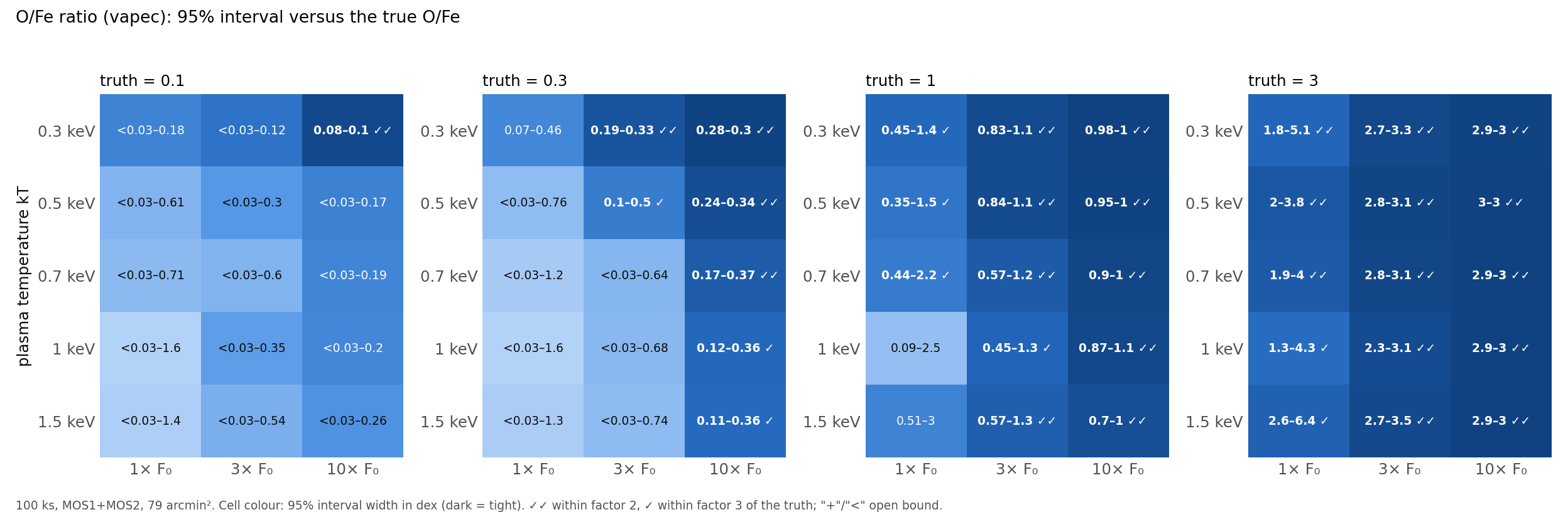
truth = 0.1
| kT | 1× F₀ | 3× F₀ | 10× F₀ |
|---|---|---|---|
| 0.3 keV | <0.03–0.18 | <0.03–0.12 | 0.08–0.10 |
| 0.5 keV | <0.03–0.61 | <0.03–0.30 | <0.03–0.17 |
| 0.7 keV | <0.03–0.71 | <0.03–0.60 | <0.03–0.19 |
| 1 keV | <0.03–1.62 | <0.03–0.35 | <0.03–0.20 |
| 1.5 keV | <0.03–1.38 | <0.03–0.54 | <0.03–0.26 |
truth = 0.3
| kT | 1× F₀ | 3× F₀ | 10× F₀ |
|---|---|---|---|
| 0.3 keV | 0.07–0.46 | 0.19–0.33 | 0.28–0.30 |
| 0.5 keV | <0.03–0.76 | 0.10–0.50 | 0.24–0.34 |
| 0.7 keV | <0.03–1.18 | <0.03–0.64 | 0.17–0.37 |
| 1 keV | <0.03–1.60 | <0.03–0.68 | 0.12–0.36 |
| 1.5 keV | <0.03–1.28 | <0.03–0.74 | 0.11–0.36 |
truth = 1
| kT | 1× F₀ | 3× F₀ | 10× F₀ |
|---|---|---|---|
| 0.3 keV | 0.45–1.37 | 0.83–1.07 | 0.98–1.01 |
| 0.5 keV | 0.35–1.48 | 0.84–1.14 | 0.95–1.01 |
| 0.7 keV | 0.44–2.17 | 0.57–1.21 | 0.90–1.03 |
| 1 keV | 0.09–2.47 | 0.45–1.27 | 0.87–1.05 |
| 1.5 keV | 0.51–3.03 | 0.57–1.34 | 0.70–1.03 |
truth = 3
| kT | 1× F₀ | 3× F₀ | 10× F₀ |
|---|---|---|---|
| 0.3 keV | 1.79–5.12 | 2.68–3.26 | 2.94–3.05 |
| 0.5 keV | 1.96–3.75 | 2.78–3.08 | 2.98–3.01 |
| 0.7 keV | 1.90–4.02 | 2.75–3.12 | 2.94–3.01 |
| 1 keV | 1.27–4.30 | 2.32–3.15 | 2.94–3.01 |
| 1.5 keV | 2.58–6.37 | 2.74–3.51 | 2.94–3.03 |
Cells that satisfy each criterion, 100 ks:
| truth | cells within a factor of 3 (95%) | cells within a factor of 2 (95%) |
|---|---|---|
| O/Fe = 0.1 | 10× F₀: kT = 0.3 | 10× F₀: kT = 0.3 |
| O/Fe = 0.3 | 3× F₀: kT = 0.3, 0.5; 10× F₀: kT = 0.3, 0.5, 0.7, 1, 1.5 | 3× F₀: kT = 0.3; 10× F₀: kT = 0.3, 0.5, 0.7 |
| O/Fe = 1 | 1× F₀: kT = 0.3, 0.5, 0.7; 3× F₀: kT = 0.3, 0.5, 0.7, 1, 1.5; 10× F₀: kT = 0.3, 0.5, 0.7, 1, 1.5 | 3× F₀: kT = 0.3, 0.5, 0.7, 1.5; 10× F₀: kT = 0.3, 0.5, 0.7, 1, 1.5 |
| O/Fe = 3 | 1× F₀: kT = 0.3, 0.5, 0.7, 1, 1.5; 3× F₀: kT = 0.3, 0.5, 0.7, 1, 1.5; 10× F₀: kT = 0.3, 0.5, 0.7, 1, 1.5 | 1× F₀: kT = 0.3, 0.5, 0.7; 3× F₀: kT = 0.3, 0.5, 0.7, 1, 1.5; 10× F₀: kT = 0.3, 0.5, 0.7, 1, 1.5 |
Reading the two maps
- Absolute Z: a low true metallicity is the easy case. At fixed broadband surface brightness, Ztrue = 0.1 leaves a bright continuum: at 1× F₀ the upper bound closes for every kT ≥ 1 keV (≤0.3 for 1.5 keV), at 3× F₀ the constraint is within a factor of 2 for kT = 1–1.5 keV, and at 10× F₀ every temperature from 0.5 to 2 keV is within a factor of 2. For Ztrue = 0.3 the factor-of-2 region starts at 3× F₀ for kT ≥ 1.5 keV and at 10× F₀ for kT ≥ 1 keV; for Ztrue = 1 it needs 3× F₀ and kT ≥ 1.5 keV, or 10× F₀ and kT ≥ 1.5 keV (kT = 1 keV at 10× F₀ reaches a factor of 3). For Ztrue = 3, with the profile grid extended to Z = 20, the upper bound stays open at 20 in every cell except kT = 2 keV (0.8–14 at 1× F₀, 2.3–8.9 at 3× F₀, 2.9–3.8 at 10× F₀) and kT = 1.5 keV at 10× F₀ (2.9–7.3): a metal-rich, line-dominated plasma has almost no continuum left to bound Z from above, which is the same shape as the Chandra bulge measurement of M104 (Z = 2.2, +1.6/−0.8).
- O/Fe: an oxygen-rich ratio is the easy case, an iron-rich one is hard. O/Fetrue = 3 is within a factor of 2 at 1× F₀ for kT ≤ 0.7 keV and at ≥3× F₀ everywhere. Solar O/Fe is within a factor of 3 at 1× F₀ for kT ≤ 0.7 keV, within a factor of 2 at 3× F₀ for most temperatures and at 10× F₀ for all. O/Fetrue = 0.3, the Type Ia-like value, is within a factor of 2 only at 3× F₀ for kT = 0.3 keV and at 10× F₀ for kT ≤ 0.7 keV, and O/Fetrue = 0.1 gives upper limits only, except for the coolest, brightest cell. Bounding a weak oxygen line from below against the fixed foreground O VII/O VIII is the hard measurement.
- For M104's inner halo (0.7 keV, 1× F₀) every true value tried gives an open-ended interval for absolute Z at 100 ks. O/Fe is bounded to within a factor of 3 if it is solar (0.44–2.2) and a factor of 2 if it is oxygen-rich (1.9–4.0 for a truth of 3), but is an upper limit only for an iron-rich ratio (<1.2 for a truth of 0.3, <0.7 for 0.1). The bulge (r < 2′, 4–10× F₀) is constrained for O/Fe at any truth ≥ 0.3 and for absolute Z only if the true Z is ≲ 0.3.
- All cells are single realizations at 100 ks; bounds move by roughly ±50% between realizations (Section 3). The maps show where a constraint exists, not its exact width.
Data: summary_ccdZ_allZtrue.csv, summary_OFe_allR.csv; per-cell profiles in the two profile folders (files with _Z or _R suffixes).
6. Exposure needed for a 0.7 keV plasma in M104's two annuli
Each annulus is simulated with its own ARF, RMF, point-source-masked sky area and quiescent particle background: R2–5′ (6.6–16.5 kpc; 36.6 + 42.3 = 79 arcmin² effective on MOS1 + MOS2, 66 arcmin² geometric) at its surface brightness of 1× F₀, and R5–9′ (16.5–30 kpc; 81.8 + 129.8 = 212 arcmin² effective, 176 arcmin² geometric) at its surface brightness of 0.3× F₀. Columns are the clean exposure of the annulus with both MOS cameras on, from 300 to 10 000 ks; the area × exposure product (effective area summed over the two cameras) is given under each column for transfer to other region sizes. True Z = 0.1, 0.3, 1 and 3; the profile grid extends to Z = 20 for true Z ≥ 1.
Three background contracts are shown, because the answer depends on how much is known about the soft protons: index and norm free per camera (the honest default), shape frozen with the norm free (what a broad in-field fit of the same observation can supply), and everything frozen (perfect background knowledge, the pure Poisson limit).
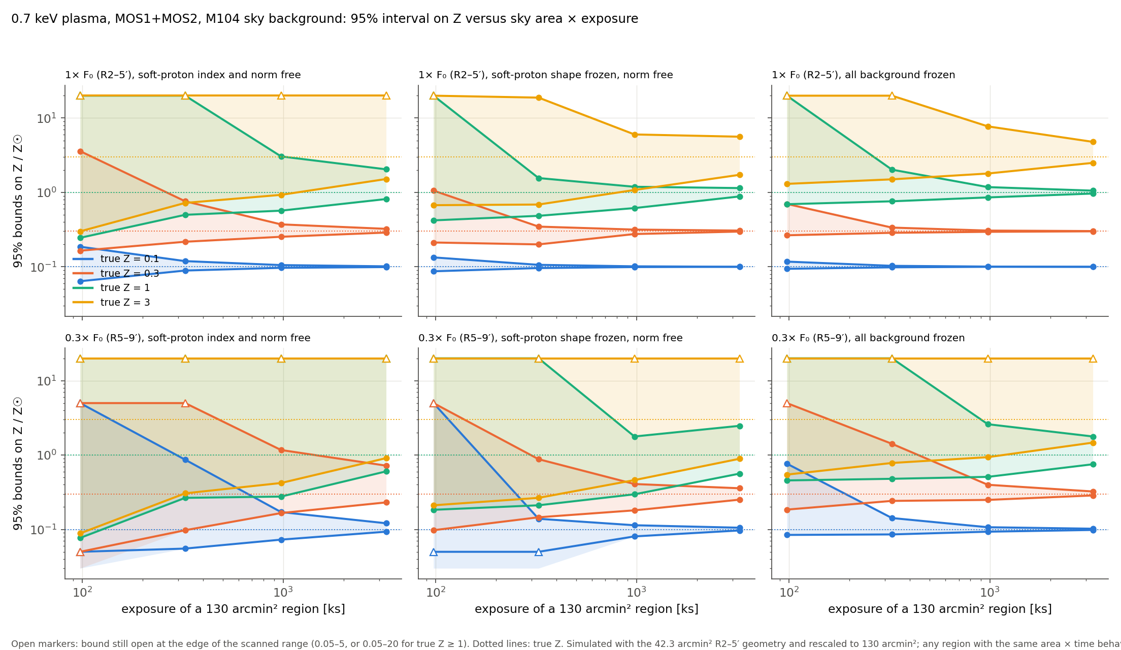
Soft-proton index and norm free
R2–5′ annulus (1× F₀, 6.6–16.5 kpc, 79 arcmin² effective)
| true Z | 300 ks on R2–5′ 23670 arcmin² ks | 1000 ks on R2–5′ 78900 arcmin² ks | 3000 ks on R2–5′ 236700 arcmin² ks | 10000 ks on R2–5′ 789000 arcmin² ks |
|---|---|---|---|---|
| 0.1 | 0.064–0.19 | 0.089–0.12 | 0.097–0.11 | 0.099–0.1 |
| 0.3 | 0.16–3.6 | 0.22–0.76 | 0.25–0.37 | 0.29–0.32 |
| 1 | 0.25–20+ | 0.5–20+ | 0.57–3.1 | 0.81–2 |
| 3 | 0.3–20+ | 0.72–20+ | 0.93–20+ | 1.5–20+ |
R5–9′ annulus (0.3× F₀, 16.5–30 kpc, 212 arcmin² effective)
| true Z | 300 ks on R5–9′ 63480 arcmin² ks | 1000 ks on R5–9′ 211600 arcmin² ks | 3000 ks on R5–9′ 634800 arcmin² ks | 10000 ks on R5–9′ 2116000 arcmin² ks |
|---|---|---|---|---|
| 0.1 | <0.05–1.3 | 0.054–0.18 | 0.089–0.14 | 0.097–0.11 |
| 0.3 | 0.093–5+ | 0.15–5+ | 0.19–0.59 | 0.26–0.44 |
| 1 | 0.16–20+ | 0.25–20+ | 0.37–20+ | 0.57–6.7 |
| 3 | 0.19–20+ | 0.31–20+ | 0.49–20+ | 0.94–20+ |
95% intervals on Z (green: within a factor of 2 of the truth; blue: within a factor of 3; grey: a bound is still open). Smallest clean exposure of the annulus (both MOS) reaching each criterion:
| annulus | true Z | within a factor of 3 | within a factor of 2 |
|---|---|---|---|
| R2–5′ | 0.1 | 300 ks | 300 ks |
| R2–5′ | 0.3 | 1000 ks | 3000 ks |
| R2–5′ | 1 | 10000 ks | not reached by 10000 ks |
| R2–5′ | 3 | not reached by 10000 ks | not reached by 10000 ks |
| R5–9′ | 0.1 | 1000 ks | 1000 ks |
| R5–9′ | 0.3 | 3000 ks | 3000 ks |
| R5–9′ | 1 | not reached by 10000 ks | not reached by 10000 ks |
| R5–9′ | 3 | not reached by 10000 ks | not reached by 10000 ks |
Soft-proton shape frozen, norm free
R2–5′ annulus (1× F₀, 6.6–16.5 kpc, 79 arcmin² effective)
| true Z | 300 ks on R2–5′ 23670 arcmin² ks | 1000 ks on R2–5′ 78900 arcmin² ks | 3000 ks on R2–5′ 236700 arcmin² ks | 10000 ks on R2–5′ 789000 arcmin² ks |
|---|---|---|---|---|
| 0.1 | 0.087–0.13 | 0.096–0.11 | 0.099–0.1 | 0.1–0.1 |
| 0.3 | 0.21–1.1 | 0.2–0.35 | 0.28–0.32 | 0.3–0.31 |
| 1 | 0.42–20+ | 0.48–1.6 | 0.62–1.2 | 0.88–1.1 |
| 3 | 0.67–20+ | 0.69–19 | 1.1–6 | 1.7–5.6 |
R5–9′ annulus (0.3× F₀, 16.5–30 kpc, 212 arcmin² effective)
| true Z | 300 ks on R5–9′ 63480 arcmin² ks | 1000 ks on R5–9′ 211600 arcmin² ks | 3000 ks on R5–9′ 634800 arcmin² ks | 10000 ks on R5–9′ 2116000 arcmin² ks |
|---|---|---|---|---|
| 0.1 | <0.05–0.18 | 0.066–0.11 | 0.096–0.11 | 0.099–0.1 |
| 0.3 | 0.13–2.2 | 0.17–0.36 | 0.22–0.37 | 0.28–0.33 |
| 1 | 0.2–20+ | 0.27–1.7 | 0.49–2.7 | 0.68–1.6 |
| 3 | 0.28–20+ | 0.37–20+ | 0.78–20+ | 1.3–20+ |
95% intervals on Z (green: within a factor of 2 of the truth; blue: within a factor of 3; grey: a bound is still open). Smallest clean exposure of the annulus (both MOS) reaching each criterion:
| annulus | true Z | within a factor of 3 | within a factor of 2 |
|---|---|---|---|
| R2–5′ | 0.1 | 300 ks | 300 ks |
| R2–5′ | 0.3 | 1000 ks | 1000 ks |
| R2–5′ | 1 | 1000 ks | 3000 ks |
| R2–5′ | 3 | 3000 ks | 10000 ks |
| R5–9′ | 0.1 | 1000 ks | 1000 ks |
| R5–9′ | 0.3 | 1000 ks | 1000 ks |
| R5–9′ | 1 | 3000 ks | 10000 ks |
| R5–9′ | 3 | not reached by 10000 ks | not reached by 10000 ks |
All background frozen
R2–5′ annulus (1× F₀, 6.6–16.5 kpc, 79 arcmin² effective)
| true Z | 300 ks on R2–5′ 23670 arcmin² ks | 1000 ks on R2–5′ 78900 arcmin² ks | 3000 ks on R2–5′ 236700 arcmin² ks | 10000 ks on R2–5′ 789000 arcmin² ks |
|---|---|---|---|---|
| 0.1 | 0.094–0.12 | 0.098–0.1 | 0.1–0.1 | 0.1–0.1 |
| 0.3 | 0.27–0.7 | 0.29–0.34 | 0.3–0.31 | 0.3–0.3 |
| 1 | 0.69–20+ | 0.76–2 | 0.86–1.2 | 0.97–1.1 |
| 3 | 1.3–20+ | 1.5–20+ | 1.8–7.7 | 2.5–4.8 |
R5–9′ annulus (0.3× F₀, 16.5–30 kpc, 212 arcmin² effective)
| true Z | 300 ks on R5–9′ 63480 arcmin² ks | 1000 ks on R5–9′ 211600 arcmin² ks | 3000 ks on R5–9′ 634800 arcmin² ks | 10000 ks on R5–9′ 2116000 arcmin² ks |
|---|---|---|---|---|
| 0.1 | 0.082–0.26 | 0.091–0.11 | 0.098–0.1 | 0.1–0.1 |
| 0.3 | 0.23–4 | 0.21–0.4 | 0.28–0.34 | 0.3–0.31 |
| 1 | 0.5–20+ | 0.47–3.3 | 0.69–2.1 | 0.88–1.4 |
| 3 | 0.82–20+ | 0.7–20+ | 1.4–20+ | 1.9–18 |
95% intervals on Z (green: within a factor of 2 of the truth; blue: within a factor of 3; grey: a bound is still open). Smallest clean exposure of the annulus (both MOS) reaching each criterion:
| annulus | true Z | within a factor of 3 | within a factor of 2 |
|---|---|---|---|
| R2–5′ | 0.1 | 300 ks | 300 ks |
| R2–5′ | 0.3 | 300 ks | 1000 ks |
| R2–5′ | 1 | 1000 ks | 3000 ks |
| R2–5′ | 3 | 3000 ks | 10000 ks |
| R5–9′ | 0.1 | 300 ks | 1000 ks |
| R5–9′ | 0.3 | 1000 ks | 1000 ks |
| R5–9′ | 1 | 3000 ks | 10000 ks |
| R5–9′ | 3 | not reached by 10000 ks | not reached by 10000 ks |
Reading the scan
- Inner annulus (R2–5′, 1× F₀), soft protons free: a true Z of 0.1 is within a factor of 2 at 300 ks; 0.3 needs 1000 ks for a factor of 3 and 3000 ks for a factor of 2; 1 needs 10000 ks for a factor of 3 and not reached by 10000 ks for a factor of 2; for 3 a factor of 3 is not reached by 10000 ks. The current data are 66 ks clean; a 500 ks raw programme gives ≈400 ks clean per camera.
- Outer annulus (R5–9′, 0.3× F₀), simulated with its own responses and background: a true Z of 0.1 is within a factor of 3 at 1000 ks and a factor of 2 at 1000 ks; 0.3 needs 3000 ks (factor 3) and 3000 ks (factor 2); for 1 a factor of 3 is not reached by 10000 ks; for 3 it is not reached by 10000 ks. The outer annulus has 2.7× the effective area of the inner one but, because of vignetting, only 2.2× the source counts at the same surface brightness and exposure; the earlier version of this section rescaled the inner-annulus simulation by area alone, which overstated the outer annulus by ≈20%, and is no longer used.
- Knowing the soft-proton shape moves a solar inner annulus to 1000 ks (factor 3) and 3000 ks (factor 2), and a super-solar one to 3000 ks (factor 3); with every background component frozen the numbers are 1000 ks / 3000 ks for Z = 1 and 3000 ks / 10000 ks for Z = 3. The lower bound is insensitive to the contract; the upper bound is what the soft-proton continuum erases.
- The scan is a single realization per point; a few cells move against the trend, which is the ±50% realization scatter seen elsewhere on this page. To transfer to a region of different size at the same surface brightness use the area × exposure products under the column headers (effective, point-source-masked area summed over the two cameras), remembering that off-axis vignetting lowers the counts per unit area.
Data: summary_grasp_kT0.7.csv. Single realizations, MOS only, sky foreground and CXB fixed. Systematic floors (CXB field-to-field scatter, soft-proton shape, multi-temperature Fe bias) do not shrink with exposure, so the longest exposures here are statistical limits that real data would not reach.
7. Caveats
- MOS only. No per-annulus pn products were available. pn adds continuum counts in 1–7 keV but also background; a √2–√3 equivalent gain would shift the boundaries in Figures 2–3 by less than one brightness step and would not make the (≤0.7 keV, ≤3× F₀) cells constrained.
- Foreground O lines fixed. For O/Fe the Local Hot Bubble and Milky Way halo (with their O VII / O VIII) are frozen at truth. In real data their normalisation (and solar-wind charge exchange) is uncertain at the 10–20% level and leaks directly into the source O; at 1× F₀ the source O-band counts are comparable to the foreground, so this systematic would dominate for a faint halo.
- Single realization per cell. Interval bounds scatter by roughly ±50% between realizations (visible as 300 ks cells that look no better than 100 ks ones). The maps show where a constraint exists, not its precise width.
- Single-temperature truth. A 30% cool-phase (0.35 keV) injection into R2–5′ fitted with one temperature biases kT to 0.53 keV and pushes Z to the start value: Fe bias and temperature bias appear together.
- Statistic.
chi2gehrelson subtracted, grouped data gives stat/dof ≈ 0.7 at truth; true Δχ² values are ≈1.4× larger, which does not change any conclusion. - Soft protons. The truth uses one power-law shape per camera (Γ ≈ 1.2–1.3, MOS2 norm scaled by 0.7 to match the observed rates); above 3.2 keV a single power law over-predicts the real spectrum, which only matters for the 0.4–7 keV grid fits and is consistent between truth and fit.
8. Data and code
- summary_ccdZ.csv — absolute-Z base grid (truth 0.5): 68% / 95% intervals, best-fit Z, source counts, Δχ² range per cell.
- summary_OFe.csv — O/Fe base grid (truth 1.0), same columns.
- summary.csv — the M104 two-zone Monte-Carlo grid (recovered Zin, Zout, kT; medians and 16–84% ranges); individual realizations in
data/results_*.csv. - summary_ccdZ_allZtrue.csv, summary_OFe_allR.csv — the truth-dependence grids of Section 5; summary_grasp_kT0.7.csv — the area × exposure scan of Section 6.
- Profiles for the M104 case: SP free, F=6, Z=1, SP free, F=6, Z=0.3, SP free, F=1, Z=0.3, SP shape frozen, all background frozen, Z=1, all background frozen, Z=0.3.
- Per-cell grid profiles: profiles_Z/, profiles_OFe/.
- Scripts (Sherpa):
fakeit_twozone_Z.py(model, fake, two-zone fit),profile_Z.py,ccd_Z_limits.py,ccd_OFe_limits.py,summarize*.py,make_figures.py,build_*.py.
Prepared 2026-09-24 and recomputed 2026-09-25 (after fixing an exposure-scaling bug: the folded model was not rebuilt after changing the exposure, which had under-counted the source in every cell with exposure ≠ 66 ks) as part of the feasibility assessment for a deep XMM-Newton observation of M104. Related published analysis of the same data: Li, Huang et al. 2026, arXiv:2609.18006.