CCD 何时能约束热晕气体的金属丰度?
基于 M104(NGC 4594,ObsID 0900170101)XMM-Newton EPIC MOS 观测的 fakeit 研究:绝对金属丰度与 O/Fe 比随等离子体温度、面亮度和曝光的变化,采用该天区的真实天空背景、软质子与仪器线模型。
2026-09-24, revised 2026-09-25XMM-Newton EPIC MOS1+MOS2Sherpa 4.18 / XSPEC 12.14 apec & vapecsingle-realization Δχ² profiles
一段话结论。 For a ~0.7 keV halo at the surface brightness of M104's inner halo (6.6–16.5 kpc, 1× F₀) the CCD spectrum gives only a lower bound on the metallicity unless the true Z is low: with the soft protons free, six times the current exposure (≈400 ks clean per camera) constrains Zin to 0.14–0.52 if the truth is 0.3, but only to Zin每个要求都大 3–10 倍:真值 Z = 0.1 需要 × 976 ks,0.3 需要 × 3254 ks 达 3 倍,Z ≥ 1 永远无法界定。400 ks 净曝光计划给 R5–9′ 提供 130 arcmin² × 400 ks,只够贫金属(Z ≈ 0.1)晕。
1. 实验设置
数据产品与几何
- ObsID 0900170101(XART-ATOMS 中心视场),MOS1 与 MOS2,ESAS 产品,点源已掩蔽。两个完整环:R2–5′(6.6–16.5 kpc;MOS1/MOS2 上分别为 36.6 与 42.3 arcmin²)和 R5–9′(16.5–30 kpc;81.8 与 129.8 arcmin²)。每相机净曝光 65.8 / 65.2 ks。每个环有自己的 ARF、RMF 与静默粒子背景(QPB)光谱。
- 提取天区面积。 The generalised grids (Sections 3–5) use the R2–5′ geometry only: 36.6 arcmin² on MOS1 and 42.3 arcmin² on MOS2 (79 arcmin² in total, the two cameras differ because of masked point sources and CCD gaps). 本页所有计数都对该面积而言。 固定面亮度下源计数随面积线性标度,因此面积为 A 的区域行为等同于本几何在 (A / 79 arcmin²) × F 面亮度下的行为;例如 20 arcmin² 区域在 4× F₀ 下的源计数与本几何在 1× F₀ 下相同,而天空、软质子与 QPB 计数也随面积标度,因此每能段的源份额不变。按总源计数(列于每张表下)读图,是把图迁移到其他区域尺寸最稳妥的方式。
- 距离标度 3.3 kpc / arcmin,与 XART-ATOMS 分析一致。pn 未包含(无逐环 pn 产品);见注意事项。
天空背景、软质子、仪器线
所有非源分量取该天区生产分析的最佳拟合值,其中天空分量由专门的偏置视场(ObsID 0900170701)固定:
| Component | Model | Value (per arcmin²) | In the fit |
|---|---|---|---|
| Local Hot Bubble | apec, kT = 0.083 keV, Z = 1 | norm 3.41 × 10⁻⁶ | fixed |
| Milky Way halo | apec, kT = 0.177 keV, Z = 0.3, absorbed | norm 4.53 × 10⁻⁶ | fixed |
| Cosmic X-ray background | pegpwrlw, Γ = 1.46, 0.5–2 keV, absorbed | 1.05 × 10⁻¹⁵ erg cm⁻² s⁻¹ | fixed (±10% variants tested) |
| Absorption | phabs | NH = 3 × 10²⁰ cm⁻² | fixed |
| Soft protons | powerlaw through RMF only (unit ARF) | Γ ≈ 1.2–1.3; norm ≈ 3.0 × 10⁻⁴ (R2–5) and 1.5 × 10⁻⁴ (R5–9) ct s⁻¹ keV⁻¹ at 1 keV, MOS1; MOS2 × 0.7 | index and norm free, per camera |
| Instrumental lines | Gaussians at 1.49, 1.75 keV (Al K, Si K) and 1.28 keV | from the production fit | norms free, per camera |
源与天空分量经 ARF × RMF × 曝光折叠;软质子分量经 RMF × 曝光折叠(单位 ARF),因此其归一化是计数率而非流量。真值模型逐能段复现 QPB 已减的观测计数率,MOS1 上 1–3%、MOS2 上 5–15%(图 4)。
源与亮度标度
- 源:红移 0.003416 处的吸收
apec(或vapec)。对 M104 情形 kT = 0.72 / 0.71 keV(R2–5 / R5–9)。apec(orvapec) at redshift 0.003416. For the M104 case kT = 0.72 / 0.71 keV (R2–5 / R5–9). - F₀ = 2.68 × 10⁻¹⁵ erg cm⁻² s⁻¹ arcmin⁻²: the absorbed 0.5–2 keV surface brightness of M104's R2–5′ annulus. The grids use 0.3×, 1×, 3× and 10× F₀. For reference, the same scale in M104 itself: 0.5–1′ ≈ 10× F₀, 1–2′ ≈ 3.7× F₀, 2–4′ ≈ 1× F₀ (from the published annular fluxes), 5–9′ ≈ 0.3× F₀.
- 对每个试探 Z 值,源归一化都重新标度,使 0.7–1.0 keV(Fe-L)源计数与观测保持相等:已知量是 Fe-L 流量,未知量是 Z。
模拟与拟合合同
- 假源光谱 = Poisson(model + F × QPB);假 QPB = Poisson(F × QPB);曝光 = F × 65.8 ks。F = 1 即当前数据;F = 4 / 5 / 6 ≈ 按 75% 清洁效率的 +300 / 400 / 500 ks 原始曝光;网格直接使用 100 ks 与 300 ks。
- 拟合:QPB 已减,0.4–3.2 keV(M104 情形)或 0.4–7 keV(网格),每 bin ≥25 计数,
chi2gehrels,levmar。自由参数:kT、norm、Z(或 Fe 与 O)、逐相机软质子指数与 norm、逐相机仪器线 norm。chi2gehrels,levmar. Free: kT, norm, Z (or Fe and O), soft-proton index and norm per camera, instrumental-line norms per camera. - Δχ² 剖面:Z(或 O/Fe)固定在网格上(Z:0.05–5;O/Fe:0.1–5);其余参数在每个网格点重新拟合。区间在 log Z 插值后按 Δχ² = 1(68%)与 4(95%)读取。"2 倍以内" 指两个 95% 界限都落在 [truth/2, 2 × truth] 内;"3 倍以内" 指都落在 [truth/3, 3 × truth] 内。第 5 节将两个判据作为真值的函数报告。
2. M104 案例:Zin 的下界,且只有当晕贫金属时才有上界
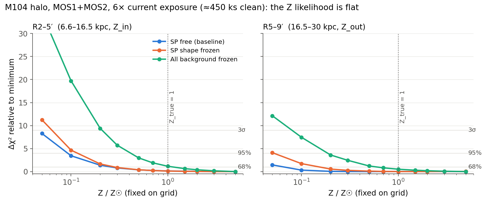
| Contract | Case | R2–5′ (Zin), 95% | R5–9′ (Zout), 95% |
|---|---|---|---|
| SP free | F = 6, Ztrue = 1 | 0.34–5+ (lower bound only; best fit at 2) | 0.30–5+ (lower bound only) |
| SP free | F = 6, Ztrue = 0.3 | 0.14–0.53 (68%: 0.18–0.31) | 0.23–5+ (lower bound only) |
| SP free | F = 1, Ztrue = 0.3 (current data) | <0.05–4.3: unconstrained | unconstrained |
| SP shape frozen | F = 6, Ztrue = 1 | 0.29–5+ (68%: 0.44–1.5) | 0.17–5+ |
| All background frozen | F = 6, Ztrue = 1 | 0.53–3.7 (68%: 0.69–1.5) | 0.33–5+ (68%: 0.48–1.8) |
| All background frozen | F = 6, Ztrue = 0.3 | 0.30–0.69 (68%: 0.42–0.54) | 0.26–2.8 (68%: 0.39–0.87) |
由此得出三点。第一,当前 66 ks 对任一环、任何真值的 Z 都无信息。第二,六倍曝光给出 Zin 的稳健下界(若晕为太阳金属丰度则 95% 下 Z > 0.3),但只有当晕贫金属时才有上界:真值 Zin = 0.3 在软质子自由时可在 2 倍以内恢复,而太阳或超太阳晕则跑出网格顶端。第三,知道背景并不定性地改变图像:所有 nuisance 分量冻结在真值时,Zin = 1 也只能界定到 0.5–3.7,且太阳晕的 Zout 仍然开放。外环(16.5–30 kpc)在任何合同下都不可测,除非其金属丰度低。每组配置八个完整两区拟合的 Monte-Carlo 网格(F = 1, 4, 6;Ztrue = 0.3, 1, 2;CXB ±10%;30% 冷相注入)在点估计上说的是同一件事:Ztrue = 0.3 时恢复的 Zin 在 F = 6 为 0.30(16–84%:0.19–0.34)、F = 4 为 0.31(0.28–0.41),Zout 分别为 0.27(0.23–0.59)与 0.24(0.18–0.40);Ztrue = 1 在 F = 6 时拟合散布在 Zin 0.64–4.6、Zout 0.31–3.2,八个 Zin 中两个与一个 Zout 落在网格边界 5,若干落在优化器起始值 1.0;Ztrue = 2 时中位数为 1.2(1.0–4.7)。kT 全程恢复到 ±0.01–0.02 keV;用单温拟合 30% 冷相注入会把 kTin 偏置到 0.67 keV、Zin 偏置到 0.57(0.38–1.6)。数据:summary.csv。
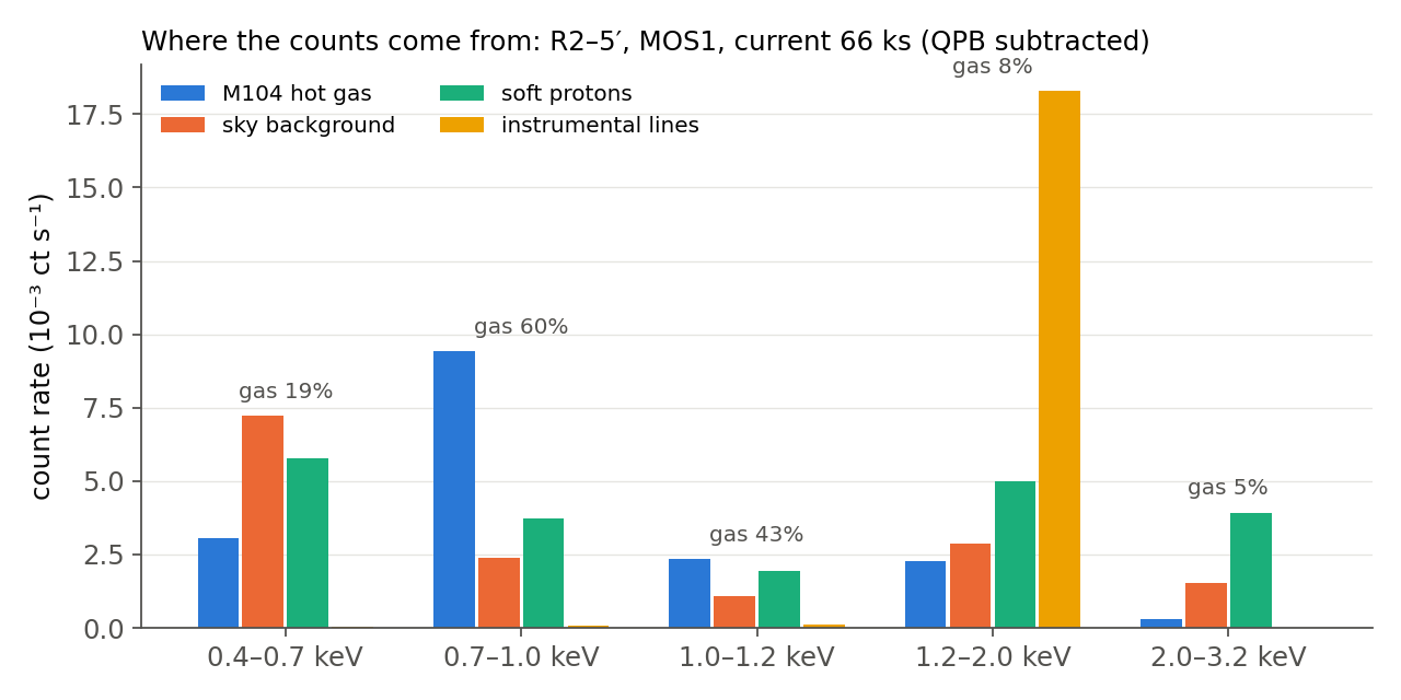
| Band (keV) | data − QPB | model total | M104 gas | sky | soft protons | lines | gas fraction |
|---|---|---|---|---|---|---|---|
| 0.4–0.7 | 15.2 | 16.1 | 3.06 | 7.24 | 5.78 | 0.05 | 19% |
| 0.7–1.0 | 15.2 | 15.6 | 9.42 | 2.40 | 3.73 | 0.07 | 60% |
| 1.0–1.2 | 5.6 | 5.5 | 2.36 | 1.07 | 1.93 | 0.11 | 43% |
| 1.2–2.0 | 28.4 | 28.4 | 2.29 | 2.87 | 4.99 | 18.28 | 8% |
| 2.0–3.2 | 5.6 | 5.8 | 0.30 | 1.53 | 3.93 | 0.02 | 5% |
计数率单位 10⁻³ ct s⁻¹,R2–5′,MOS1,QPB 已减;所有分量同单位。
3. 绝对金属丰度:温度 × 面亮度 × 曝光(真值 Z = 0.5)
本节全部假设真金属丰度 Z = 0.5 Z☉,每格单一实现,MOS1+MOS2,79 arcmin²,M104 天空背景,软质子自由,0.4–7 keV。第 5 节对真值 Z = 0.1、0.3、1 和 3 重复 100 ks 网格,因为答案取决于真值:固定 Fe-L 流量下,更低的真值 Z 意味着更亮的连续谱和更容易的上界。☉, a single realization per cell, MOS1+MOS2, 79 arcmin², M104 sky background, soft protons free, 0.4–7 keV. Section 5 repeats the 100 ks grid for true Z = 0.1, 0.3, 1 and 3, because the answer depends on the truth: at fixed Fe-L flux a lower true Z means a brighter continuum and an easier upper bound.
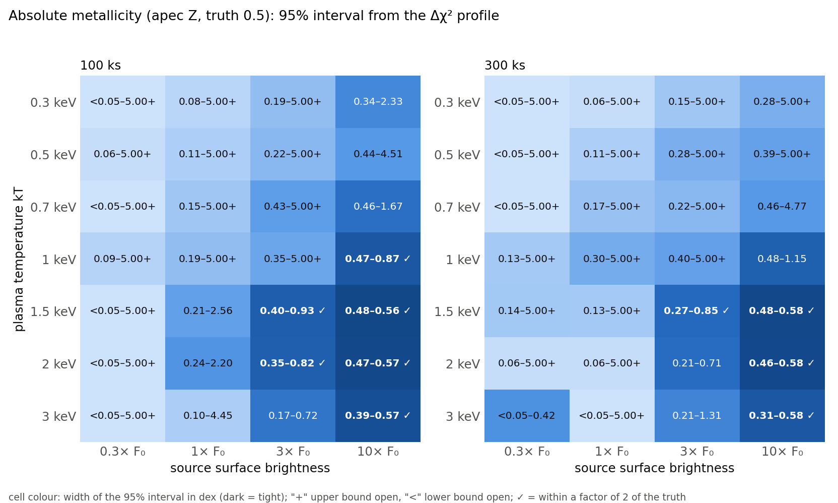
100 ks — true Z = 0.5, 95% interval on Z
| kT | 0.3× F₀ | 1× F₀ | 3× F₀ | 10× F₀ |
|---|---|---|---|---|
| 0.3 keV | unconstrained | 0.09–5.00+ | 0.20–5.00+ | 0.37–0.95 |
| 0.5 keV | 0.09–5.00+ | 0.22–5.00+ | 0.34–5.00+ | 0.47–2.53 |
| 0.7 keV | unconstrained | 0.21–5.00+ | 0.33–5.00+ | 0.47–1.18 |
| 1 keV | 0.15–5.00+ | 0.28–5.00+ | 0.41–2.65 | 0.49–0.82 |
| 1.5 keV | 0.08–5.00+ | 0.24–2.06 | 0.42–0.72 | 0.49–0.51 |
| 2 keV | unconstrained | 0.22–1.40 | 0.36–0.65 | 0.49–0.53 |
| 3 keV | unconstrained | 0.22–2.74 | 0.22–0.76 | 0.43–0.54 |
300 ks — true Z = 0.5, 95% interval on Z
| kT | 0.3× F₀ | 1× F₀ | 3× F₀ | 10× F₀ |
|---|---|---|---|---|
| 0.3 keV | 0.07–5.00+ | 0.23–5.00+ | 0.37–5.00+ | 0.47–0.78 |
| 0.5 keV | 0.06–5.00+ | 0.18–5.00+ | 0.30–1.28 | 0.48–0.72 |
| 0.7 keV | 0.07–5.00+ | 0.19–5.00+ | 0.36–1.22 | 0.49–0.65 |
| 1 keV | 0.12–5.00+ | 0.27–1.85 | 0.44–0.74 | 0.50–0.57 |
| 1.5 keV | 0.14–4.89 | 0.36–0.80 | 0.48–0.56 | 0.50–0.51 |
| 2 keV | 0.08–1.00 | 0.27–0.66 | 0.47–0.55 | 0.50–0.50 |
| 3 keV | <0.05–4.67 | 0.19–1.08 | 0.42–0.66 | 0.49–0.51 |
绿色 = 95% 下 2 倍以内,蓝色 = 3 倍以内,灰色 = 有一个界开放。summary_ccdZ.csv; per-cell profiles in data/profiles_Z/.
如何读图
- 温度是一阶控制量。 For kT ≤ 1 keV at 100 ks, Z has only a lower bound unless the surface brightness reaches 10× F₀ (and even there 0.5 keV gas gives 0.47–2.5). 剖面随 Z 单调下降:拟合倾向把连续谱交给自由的软质子分量、让源变成纯线发射,因此最小值落在上边界。
- 对 kT ≥ 1.5 keV,轫致辐射延伸到 2–7 keV 且出现 Fe K:3× F₀ 下 100 ks 足以给出 2 倍约束,1× F₀ 下 300 ks 可以(1.5 keV 时 0.36–0.80,2 keV 时 0.27–0.66)。kT = 1 keV 是过渡情形:10× F₀ 下 100 ks 或 3× F₀ 下 300 ks 达到 2 倍。
- 曝光只在连续谱可探测处有帮助,否则没有。从 100 到 300 ks 使(1× F₀,kT ≥ 1.5 keV)与(3× F₀,kT = 0.5–1 keV)的格子进入受约束区,但所有 kT ≤ 0.7 keV 且 ≤3× F₀ 的格子仍然开放。第 6 节把 0.7 keV 情形推到更大的面积 × 曝光乘积。
- M104 的内晕位于(0.7 keV,1× F₀)格:100 ks 时 0.21–5+,300 ks 时 0.19–5+。其外晕(0.3× F₀)除 2 keV、300 ks 外在任何温度都无约束。
- 单一实现:若干 300 ks 格子看起来不比对应的 100 ks 好(如 1× F₀ 的 3 keV),这是区间界 ±50% 左右的实现散布,不是趋势。
4. 线对线:vapec 的 O/Fe 比(真值 O/Fe = 1.0)
本节全部假设真 O/Fe = 1.0(Fe = O = 0.5 Z☉),几何、背景与曝光约定与第 3 节相同。第 5 节对真值 O/Fe = 0.1、0.3 和 3 重复 100 ks 网格。 (Fe = O = 0.5 Z☉), same geometry, background and exposure conventions as Section 3. Section 5 repeats the 100 ks grid for true O/Fe = 0.1, 0.3 and 3.
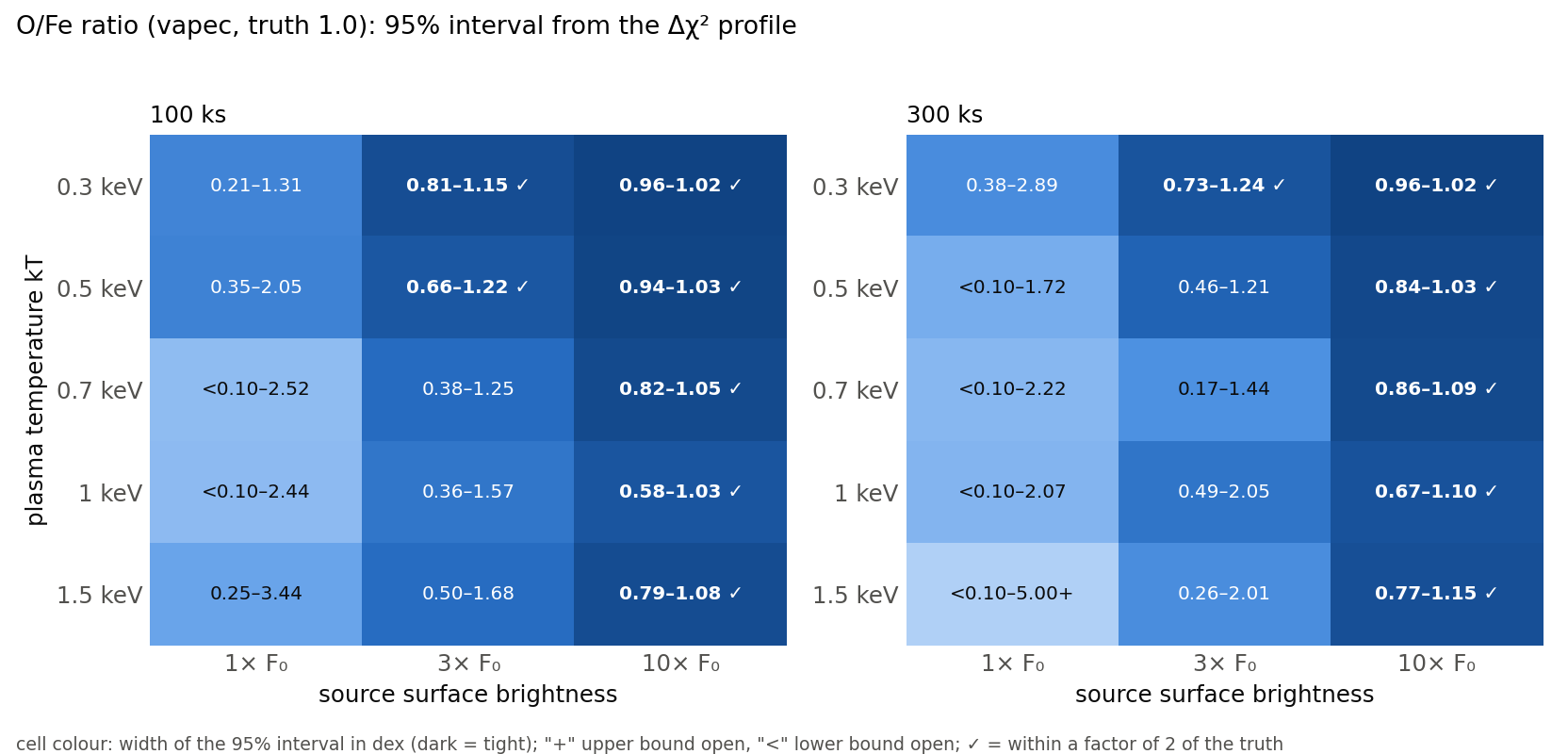
vapec Δχ² 剖面给出的 O/Fe 的 95% 区间(真值 1.0):Fe 自由(Ni 绑定)、O 自由(C、N、Ne、Mg、Al、Si、S、Ar、Ca 绑定到 O)、kT 与 norm 自由、软质子与线自由。Local Hot Bubble 与银河系晕的前景 O VII / O VIII 冻结在真值(乐观假设,见注意事项)。vapec: Fe free (Ni tied), O free (C, N, Ne, Mg, Al, Si, S, Ar, Ca tied to O), kT and norm free, soft protons and lines free. Local Hot Bubble 与银河系晕的前景 O VII / O VIII 固定在真值(乐观假设,见注意事项)。100 ks — true O/Fe = 1.0, 95% interval on O/Fe
| kT | 1× F₀ | 3× F₀ | 10× F₀ |
|---|---|---|---|
| 0.3 keV | 0.45–1.37 | 0.83–1.07 | 0.98–1.01 |
| 0.5 keV | 0.35–1.48 | 0.84–1.14 | 0.95–1.01 |
| 0.7 keV | 0.44–2.17 | 0.57–1.21 | 0.90–1.03 |
| 1 keV | 0.09–2.47 | 0.45–1.27 | 0.87–1.05 |
| 1.5 keV | 0.51–3.03 | 0.57–1.34 | 0.70–1.03 |
300 ks — true O/Fe = 1.0, 95% interval on O/Fe
| kT | 1× F₀ | 3× F₀ | 10× F₀ |
|---|---|---|---|
| 0.3 keV | 0.85–1.21 | 0.97–1.02 | 0.99–1.00 |
| 0.5 keV | 0.60–1.25 | 0.92–1.03 | 0.99–1.00 |
| 0.7 keV | 0.19–1.25 | 0.79–1.05 | 0.97–1.01 |
| 1 keV | 0.07–1.34 | 0.54–1.03 | 0.97–1.00 |
| 1.5 keV | <0.03–1.18 | 0.84–1.11 | 0.96–1.00 |
Source counts (both cameras, 100 ks, 1× F₀): 300–1100 in the O band (0.5–0.7 keV), 850–2040 in the Fe-L band. Full table: summary_OFe.csv; per-cell profiles in data/profiles_OFe/.
如何读图
- O/Fe 是远优于绝对 Z 的 CCD 观测量因为两端都是发射线,且都不依赖被软质子主导的连续谱。它恰在绝对 Z 失效处受约束:冷气体(kT ≤ 0.7 keV)在 3× F₀、100 ks 达到 ±10–30%,每个 kT ≤ 1.5 keV 在 10× F₀ 达到 ±3–15%。两张图几乎互补:绝对 Z 要热气体,O/Fe 要有强 O VIII 的冷气体。
- 对 M104 的内晕(0.7 keV,1× F₀),太阳 O/Fe 在 100 ks 界定为 0.44–2.2(3 倍以内)、300 ks 为 0.19–1.25:可以排除强 α 增丰气体,300 ks 时开始把 Type Ia 信号(O/Fe ≈ 0.3)与太阳值区分开,但前提是前景氧线已知(见注意事项)。
- M104's bulge (r < 2′, 4–10× F₀) is in the constrained region: O/Fe to ±10–20% in 100 ks, consistent with the ±0.5 obtained from 200 ks of Chandra within 5′ in the literature. 绝对 Fe 在多数格子仍无约束(最佳拟合 Fe 在边界)。
5. 对真值的依赖:哪里约束在 3 倍以内,或 2 倍以内?
第 3–4 节把真值固定在 Z = 0.5 和 O/Fe = 1。因为每个试探光谱都归一到同一 Fe-L 流量,更高的真值 Z 意味着更暗的连续谱(norm ∝ 1/Z):真值升高时上界更难、下界更容易,低真值则相反。下面的网格对 Ztrue = 0.1、0.3、1 和 3(连同第 3 节的 Z = 0.5 网格)以及 O/Fetrue = 0.1、0.3 和 3(连同第 4 节的 O/Fe = 1 网格)重复 100 ks 剖面。提取面积 79 arcmin²(36.6 + 42.3 arcmin²,MOS1 + MOS2),M104 天空背景,软质子自由。Z 剖面网格对 Ztrue ≤ 1 跑 0.05–5、对 Ztrue = 3 跑 0.05–20(XSPEC apec 的丰度上限为 5,因此扩展跑用 vapec 并把所有金属与 Fe 绑定,即同一模型);O/Fe 网格对 O/Fetrue = 1 跑 0.1–5、其余真值跑 0.03–10。开放界("+" 或 "<")因此意味着剖面在扫描范围边缘仍在最小值的 Δχ² = 4 以内。标记两个判据:✓✓ 两个 95% 界都在 [truth/2, 2 × truth] 内和✓ 都在 [truth/3, 3 × truth] 内。true = 0.1, 0.3, 1 and 3 (with the Z = 0.5 grid from Section 3) and O/Fetrue = 0.1, 0.3 and 3 (with the O/Fe = 1 grid from Section 4). Extraction area 79 arcmin² (36.6 + 42.3 arcmin², MOS1 + MOS2), M104 sky background, soft protons free. The Z profile grid runs 0.05–5 for Ztrue ≤ 1 and 0.05–20 for Ztrue = 3 (XSPEC apec caps its abundance at 5, so the extended runs use vapec with every metal tied to Fe, which is the same model); the O/Fe grid runs 0.1–5 for O/Fetrue = 1 and 0.03–10 for the other truths. An open bound ("+" or "<") therefore means the profile is still within Δχ² = 4 of its minimum at the edge of the scanned range. 标记两个判据: ✓✓ both 95% bounds within [truth/2, 2 × truth] and ✓ both within [truth/3, 3 × truth].
绝对金属丰度
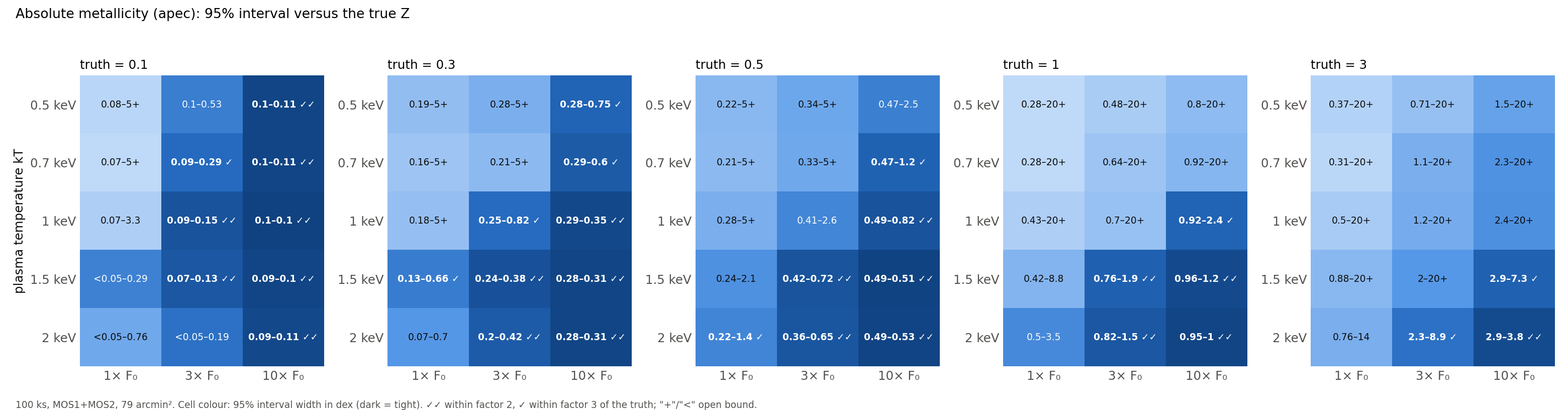
truth = 0.1
| kT | 1× F₀ | 3× F₀ | 10× F₀ |
|---|---|---|---|
| 0.5 keV | 0.08–5.00+ | 0.10–0.53 | 0.10–0.11 |
| 0.7 keV | 0.07–5.00+ | 0.09–0.29 | 0.10–0.11 |
| 1 keV | 0.07–3.26 | 0.09–0.15 | 0.10–0.10 |
| 1.5 keV | <0.05–0.29 | 0.07–0.13 | 0.09–0.10 |
| 2 keV | <0.05–0.76 | <0.05–0.19 | 0.09–0.11 |
truth = 0.3
| kT | 1× F₀ | 3× F₀ | 10× F₀ |
|---|---|---|---|
| 0.5 keV | 0.19–5.00+ | 0.28–5.00+ | 0.28–0.75 |
| 0.7 keV | 0.16–5.00+ | 0.21–5.00+ | 0.29–0.60 |
| 1 keV | 0.18–5.00+ | 0.25–0.82 | 0.29–0.35 |
| 1.5 keV | 0.13–0.66 | 0.24–0.38 | 0.28–0.31 |
| 2 keV | 0.07–0.70 | 0.20–0.42 | 0.28–0.31 |
truth = 0.5
| kT | 1× F₀ | 3× F₀ | 10× F₀ |
|---|---|---|---|
| 0.5 keV | 0.22–5.00+ | 0.34–5.00+ | 0.47–2.53 |
| 0.7 keV | 0.21–5.00+ | 0.33–5.00+ | 0.47–1.18 |
| 1 keV | 0.28–5.00+ | 0.41–2.65 | 0.49–0.82 |
| 1.5 keV | 0.24–2.06 | 0.42–0.72 | 0.49–0.51 |
| 2 keV | 0.22–1.40 | 0.36–0.65 | 0.49–0.53 |
truth = 1
| kT | 1× F₀ | 3× F₀ | 10× F₀ |
|---|---|---|---|
| 0.5 keV | 0.28–20.00+ | 0.48–20.00+ | 0.80–20.00+ |
| 0.7 keV | 0.28–20.00+ | 0.64–20.00+ | 0.92–20.00+ |
| 1 keV | 0.43–20.00+ | 0.70–20.00+ | 0.92–2.41 |
| 1.5 keV | 0.42–8.76 | 0.76–1.86 | 0.96–1.22 |
| 2 keV | 0.50–3.50 | 0.82–1.53 | 0.95–1.04 |
truth = 3
| kT | 1× F₀ | 3× F₀ | 10× F₀ |
|---|---|---|---|
| 0.5 keV | 0.37–20.00+ | 0.71–20.00+ | 1.53–20.00+ |
| 0.7 keV | 0.31–20.00+ | 1.12–20.00+ | 2.27–20.00+ |
| 1 keV | 0.50–20.00+ | 1.17–20.00+ | 2.41–20.00+ |
| 1.5 keV | 0.88–20.00+ | 2.00–20.00+ | 2.93–7.31 |
| 2 keV | 0.76–13.74 | 2.34–8.89 | 2.88–3.78 |
满足各判据的单元格,100 ks:
| truth | cells within a factor of 3 (95%) | cells within a factor of 2 (95%) |
|---|---|---|
| Z = 0.1 | 3× F₀: kT = 0.7, 1, 1.5; 10× F₀: kT = 0.5, 0.7, 1, 1.5, 2 | 3× F₀: kT = 1, 1.5; 10× F₀: kT = 0.5, 0.7, 1, 1.5, 2 |
| Z = 0.3 | 1× F₀: kT = 1.5; 3× F₀: kT = 1, 1.5, 2; 10× F₀: kT = 0.5, 0.7, 1, 1.5, 2 | 3× F₀: kT = 1.5, 2; 10× F₀: kT = 1, 1.5, 2 |
| Z = 0.5 | 1× F₀: kT = 2; 3× F₀: kT = 1.5, 2; 10× F₀: kT = 0.7, 1, 1.5, 2 | 3× F₀: kT = 1.5, 2; 10× F₀: kT = 1, 1.5, 2 |
| Z = 1 | 3× F₀: kT = 1.5, 2; 10× F₀: kT = 1, 1.5, 2 | 3× F₀: kT = 1.5, 2; 10× F₀: kT = 1.5, 2 |
| Z = 3 | 3× F₀: kT = 2; 10× F₀: kT = 1.5, 2 | 10× F₀: kT = 2 |
O/Fe 比
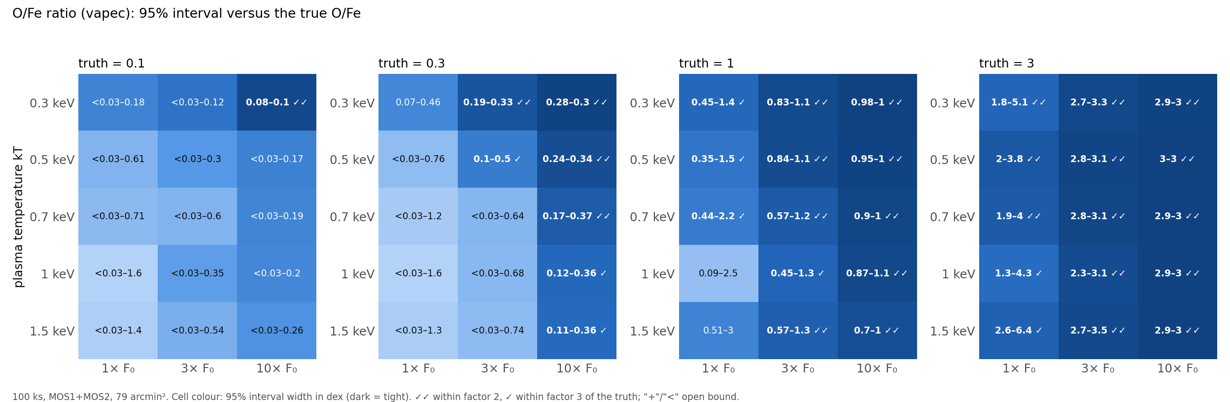
truth = 0.1
| kT | 1× F₀ | 3× F₀ | 10× F₀ |
|---|---|---|---|
| 0.3 keV | <0.03–0.18 | <0.03–0.12 | 0.08–0.10 |
| 0.5 keV | <0.03–0.61 | <0.03–0.30 | <0.03–0.17 |
| 0.7 keV | <0.03–0.71 | <0.03–0.60 | <0.03–0.19 |
| 1 keV | <0.03–1.62 | <0.03–0.35 | <0.03–0.20 |
| 1.5 keV | <0.03–1.38 | <0.03–0.54 | <0.03–0.26 |
truth = 0.3
| kT | 1× F₀ | 3× F₀ | 10× F₀ |
|---|---|---|---|
| 0.3 keV | 0.07–0.46 | 0.19–0.33 | 0.28–0.30 |
| 0.5 keV | <0.03–0.76 | 0.10–0.50 | 0.24–0.34 |
| 0.7 keV | <0.03–1.18 | <0.03–0.64 | 0.17–0.37 |
| 1 keV | <0.03–1.60 | <0.03–0.68 | 0.12–0.36 |
| 1.5 keV | <0.03–1.28 | <0.03–0.74 | 0.11–0.36 |
truth = 1
| kT | 1× F₀ | 3× F₀ | 10× F₀ |
|---|---|---|---|
| 0.3 keV | 0.45–1.37 | 0.83–1.07 | 0.98–1.01 |
| 0.5 keV | 0.35–1.48 | 0.84–1.14 | 0.95–1.01 |
| 0.7 keV | 0.44–2.17 | 0.57–1.21 | 0.90–1.03 |
| 1 keV | 0.09–2.47 | 0.45–1.27 | 0.87–1.05 |
| 1.5 keV | 0.51–3.03 | 0.57–1.34 | 0.70–1.03 |
truth = 3
| kT | 1× F₀ | 3× F₀ | 10× F₀ |
|---|---|---|---|
| 0.3 keV | 1.79–5.12 | 2.68–3.26 | 2.94–3.05 |
| 0.5 keV | 1.96–3.75 | 2.78–3.08 | 2.98–3.01 |
| 0.7 keV | 1.90–4.02 | 2.75–3.12 | 2.94–3.01 |
| 1 keV | 1.27–4.30 | 2.32–3.15 | 2.94–3.01 |
| 1.5 keV | 2.58–6.37 | 2.74–3.51 | 2.94–3.03 |
满足各判据的单元格,100 ks:
| truth | cells within a factor of 3 (95%) | cells within a factor of 2 (95%) |
|---|---|---|
| O/Fe = 0.1 | 10× F₀: kT = 0.3 | 10× F₀: kT = 0.3 |
| O/Fe = 0.3 | 3× F₀: kT = 0.3, 0.5; 10× F₀: kT = 0.3, 0.5, 0.7, 1, 1.5 | 3× F₀: kT = 0.3; 10× F₀: kT = 0.3, 0.5, 0.7 |
| O/Fe = 1 | 1× F₀: kT = 0.3, 0.5, 0.7; 3× F₀: kT = 0.3, 0.5, 0.7, 1, 1.5; 10× F₀: kT = 0.3, 0.5, 0.7, 1, 1.5 | 3× F₀: kT = 0.3, 0.5, 0.7, 1.5; 10× F₀: kT = 0.3, 0.5, 0.7, 1, 1.5 |
| O/Fe = 3 | 1× F₀: kT = 0.3, 0.5, 0.7, 1, 1.5; 3× F₀: kT = 0.3, 0.5, 0.7, 1, 1.5; 10× F₀: kT = 0.3, 0.5, 0.7, 1, 1.5 | 1× F₀: kT = 0.3, 0.5, 0.7; 3× F₀: kT = 0.3, 0.5, 0.7, 1, 1.5; 10× F₀: kT = 0.3, 0.5, 0.7, 1, 1.5 |
如何读这两张图
- 绝对 Z:低真值金属丰度是容易的情形。固定 Fe-L 流量下,Ztrue = 0.1 留下亮连续谱:1× F₀ 时每个 kT ≥ 1 keV 的上界都闭合(1.5 keV 时 ≤0.3),3× F₀ 时 kT = 1–1.5 keV 在 2 倍以内,10× F₀ 时 0.5 到 2 keV 的每个温度都在 2 倍以内。Ztrue = 0.3 的 2 倍区从 3× F₀、kT ≥ 1.5 keV 开始,以及 10× F₀、kT ≥ 1 keV;Ztrue = 1 需要 3× F₀ 且 kT ≥ 1.5 keV,或 10× F₀ 且 kT ≥ 1.5 keV(kT = 1 keV 在 10× F₀ 达到 3 倍)。Ztrue = 3 在剖面网格扩展到 Z = 20 后,除 kT = 2 keV(1× F₀ 时 0.8–14,3× F₀ 时 2.3–8.9,10× F₀ 时 2.9–3.8)与 10× F₀ 的 kT = 1.5 keV(2.9–7.3)外,每个格子的上界在 20 处仍开放:富金属、线主导的等离子体几乎没有留下可以从上方界定 Z 的连续谱,这与 M104 核球的 Chandra 测量(Z = 2.2, +1.6/−0.8)形状相同。
- O/Fe:富氧比是容易的情形,富铁比则难。O/Fetrue = 3 在 1× F₀、kT ≤ 0.7 keV 以及 ≥3× F₀ 的所有温度都在 2 倍以内。太阳 O/Fe 在 1× F₀、kT ≤ 0.7 keV 为 3 倍以内,3× F₀ 多数温度与 10× F₀ 全部温度为 2 倍以内。O/Fetrue = 0.3(Type Ia 型值)只在 3× F₀、kT = 0.3 keV 与 10× F₀、kT ≤ 0.7 keV 达到 2 倍以内;O/Fetrue = 0.1 除最冷最亮的格子外只给上限。对着固定的前景 O VII/O VIII 从下方界定一条弱氧线,是难的测量。
- 对 M104 的内晕(0.7 keV,1× F₀),所有试过的真值在 100 ks 都给出开放区间(绝对 Z)。O/Fe 在太阳值时 3 倍以内(0.44–2.2)、富氧值时 2 倍以内(真值 3 时 1.9–4.0),但富铁比只给上限(真值 0.3 时 <1.2,0.1 时 <0.7)。核球(r < 2′,4–10× F₀)对任何真值 ≥ 0.3 的 O/Fe 都受约束,而绝对 Z 只在真值 Z ≲ 0.3 时受约束。
- 所有格子都是 100 ks 的单一实现;实现之间界限移动约 ±50%(第 3 节)。这些图显示约束存在于何处,不显示其精确宽度。
Data: summary_ccdZ_allZtrue.csv, summary_OFe_allR.csv; per-cell profiles in the two profile folders (files with _Z or _R suffixes).
6. M104 面亮度下 0.7 keV 等离子体所需的天区面积 × 曝光
固定面亮度下,光谱的每个分量(热气体、天空背景、软质子、QPB、仪器线)都随天区面积与曝光的乘积标度,因此该乘积是 Poisson 极限约束的唯一变量。结果写成130 arcmin² 区域的曝光,130 arcmin² 是 M104 R5–9′ 环的 MOS2 有效天区面积(MOS1 81.8 arcmin²,几何 176 arcmin²),双 MOS 相机同开。任何面积 × 时间相同的区域行为相同:42 arcmin² × 1000 ks = 130 arcmin² × 323 ks,100 arcmin² × 400 ks = 130 arcmin² × 308 ks。模拟用 R2–5′ 几何(MOS2 有效面积 42.3 arcmin²,MOS1 36.6,几何 66)在 300–10 000 ks,并归一到 130 arcmin²。当前 M104 数据对应 R2–5′ 的 130 arcmin² × 21 ks 与 R5–9′ 的 130 arcmin² × 65 ks。130 arcmin² region, 130 arcmin² being the MOS2 effective sky area of the R5–9′ annulus of M104 (MOS1 81.8 arcmin², geometric 176 arcmin²), with both MOS cameras on. 任何面积 × 时间相同的区域行为相同:42 arcmin² × 1000 ks = 130 arcmin² × 323 ks,100 arcmin² × 400 ks = 130 arcmin² × 308 ks。模拟用 R2–5′ 几何(MOS2 有效面积 42.3 arcmin²,MOS1 36.6,几何 66)在 300–10 000 ks,并归一到 130 arcmin²。当前 M104 数据对应 R2–5′ 的 130 arcmin² × 21 ks 与 R5–9′ 的 130 arcmin² × 65 ks。
展示三种背景合同,因为答案取决于对软质子知道多少:逐相机指数与 norm 自由(诚实的默认)、形状冻结而 norm 自由(同观测的宽视场内拟合所能提供的)、全部冻结(完美的背景知识,纯 Poisson 极限)。两个面亮度水平:1× F₀(R2–5′,6.6–16.5 kpc)与 0.3× F₀(R5–9′,16.5–30 kpc)。真值 Z = 0.1、0.3、1 和 3。对真值 Z ≥ 1,扫描延伸到 Z = 20。
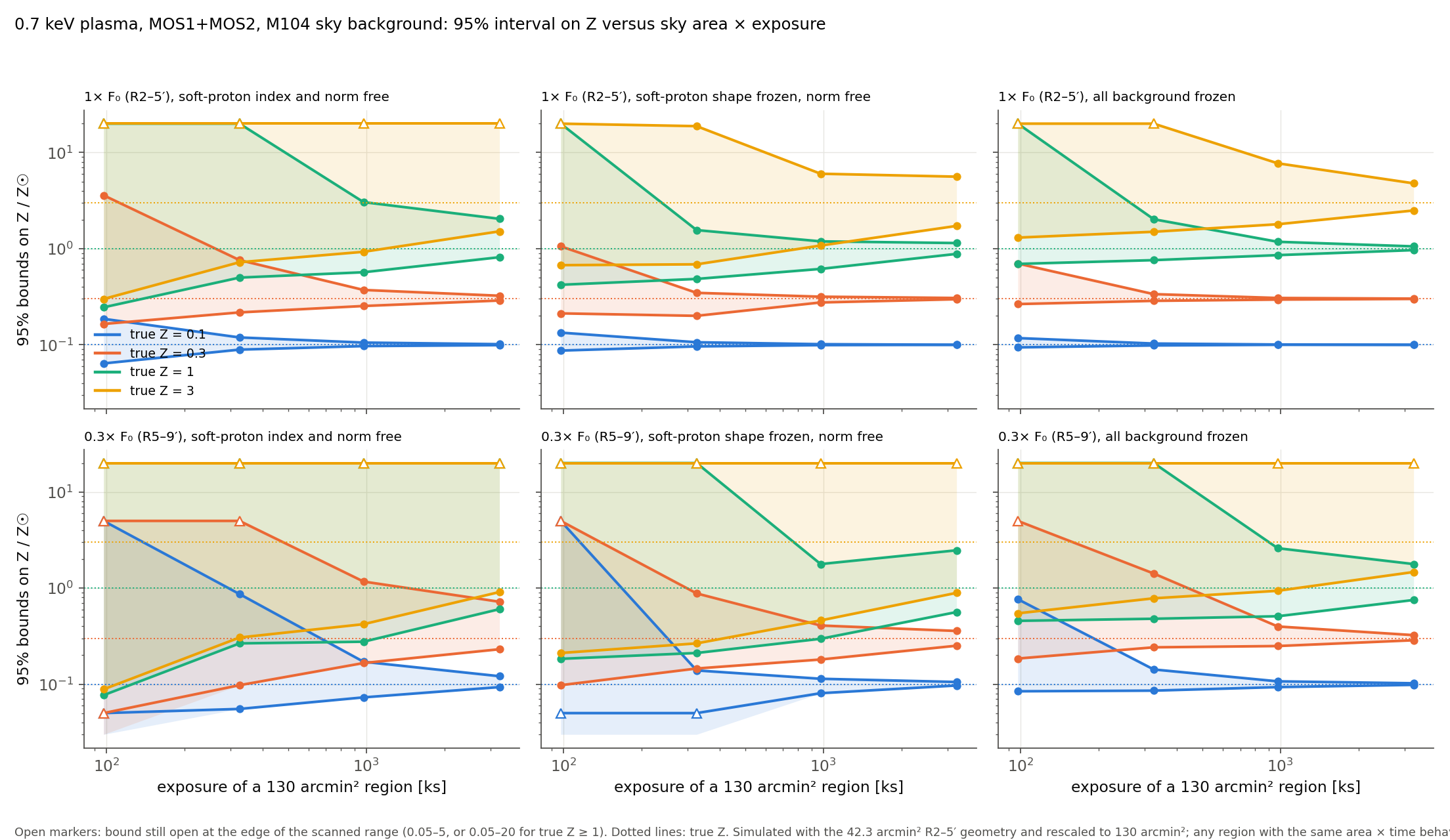
软质子指数与归一化自由
1× F₀ (R2–5′ surface brightness)
| true Z | 130 arcmin² × 98 ks simulated as 42 arcmin² × 300 ks | 130 arcmin² × 325 ks simulated as 42 arcmin² × 1000 ks | 130 arcmin² × 976 ks simulated as 42 arcmin² × 3000 ks | 130 arcmin² × 3254 ks simulated as 42 arcmin² × 10000 ks |
|---|---|---|---|---|
| 0.1 | 0.064–0.19 | 0.089–0.12 | 0.097–0.11 | 0.099–0.1 |
| 0.3 | 0.16–3.6 | 0.22–0.76 | 0.25–0.37 | 0.29–0.32 |
| 1 | 0.25–20+ | 0.5–20+ | 0.57–3.1 | 0.81–2 |
| 3 | 0.3–20+ | 0.72–20+ | 0.93–20+ | 1.5–20+ |
0.3× F₀ (R5–9′ surface brightness)
| true Z | 130 arcmin² × 98 ks simulated as 42 arcmin² × 300 ks | 130 arcmin² × 325 ks simulated as 42 arcmin² × 1000 ks | 130 arcmin² × 976 ks simulated as 42 arcmin² × 3000 ks | 130 arcmin² × 3254 ks simulated as 42 arcmin² × 10000 ks |
|---|---|---|---|---|
| 0.1 | <0.05–5+ | 0.055–0.87 | 0.073–0.17 | 0.093–0.12 |
| 0.3 | <0.05–5+ | 0.098–5+ | 0.17–1.2 | 0.23–0.72 |
| 1 | 0.077–20+ | 0.27–20+ | 0.28–20+ | 0.6–20+ |
| 3 | 0.088–20+ | 0.31–20+ | 0.42–20+ | 0.91–20+ |
95% intervals on Z (green: within a factor of 2 of the truth; blue: within a factor of 3; grey: a bound is still open). Smallest area × exposure reaching each criterion:
| brightness | true Z | smallest 130 arcmin² × t within a factor of 3 | within a factor of 2 |
|---|---|---|---|
| 1× F₀ (R2–5′) | 0.1 | 130 arcmin² × 98 ks | 130 arcmin² × 98 ks |
| 1× F₀ (R2–5′) | 0.3 | 130 arcmin² × 325 ks | 130 arcmin² × 976 ks |
| 1× F₀ (R2–5′) | 1 | 130 arcmin² × 3254 ks | not reached by 130 arcmin² × 3254 ks |
| 1× F₀ (R2–5′) | 3 | not reached by 130 arcmin² × 3254 ks | not reached by 130 arcmin² × 3254 ks |
| 0.3× F₀ (R5–9′) | 0.1 | 130 arcmin² × 976 ks | 130 arcmin² × 976 ks |
| 0.3× F₀ (R5–9′) | 0.3 | 130 arcmin² × 3254 ks | not reached by 130 arcmin² × 3254 ks |
| 0.3× F₀ (R5–9′) | 1 | not reached by 130 arcmin² × 3254 ks | not reached by 130 arcmin² × 3254 ks |
| 0.3× F₀ (R5–9′) | 3 | not reached by 130 arcmin² × 3254 ks | not reached by 130 arcmin² × 3254 ks |
Soft-proton shape frozen, norm free
1× F₀ (R2–5′ surface brightness)
| true Z | 130 arcmin² × 98 ks simulated as 42 arcmin² × 300 ks | 130 arcmin² × 325 ks simulated as 42 arcmin² × 1000 ks | 130 arcmin² × 976 ks simulated as 42 arcmin² × 3000 ks | 130 arcmin² × 3254 ks simulated as 42 arcmin² × 10000 ks |
|---|---|---|---|---|
| 0.1 | 0.087–0.13 | 0.096–0.11 | 0.099–0.1 | 0.1–0.1 |
| 0.3 | 0.21–1.1 | 0.2–0.35 | 0.28–0.32 | 0.3–0.31 |
| 1 | 0.42–20+ | 0.48–1.6 | 0.62–1.2 | 0.88–1.1 |
| 3 | 0.67–20+ | 0.69–19 | 1.1–6 | 1.7–5.6 |
0.3× F₀ (R5–9′ surface brightness)
| true Z | 130 arcmin² × 98 ks simulated as 42 arcmin² × 300 ks | 130 arcmin² × 325 ks simulated as 42 arcmin² × 1000 ks | 130 arcmin² × 976 ks simulated as 42 arcmin² × 3000 ks | 130 arcmin² × 3254 ks simulated as 42 arcmin² × 10000 ks |
|---|---|---|---|---|
| 0.1 | <0.05–5+ | <0.05–0.14 | 0.081–0.11 | 0.097–0.11 |
| 0.3 | 0.098–5+ | 0.15–0.88 | 0.18–0.41 | 0.25–0.36 |
| 1 | 0.18–20+ | 0.21–20+ | 0.3–1.8 | 0.56–2.5 |
| 3 | 0.21–20+ | 0.27–20+ | 0.46–20+ | 0.89–20+ |
95% intervals on Z (green: within a factor of 2 of the truth; blue: within a factor of 3; grey: a bound is still open). Smallest area × exposure reaching each criterion:
| brightness | true Z | smallest 130 arcmin² × t within a factor of 3 | within a factor of 2 |
|---|---|---|---|
| 1× F₀ (R2–5′) | 0.1 | 130 arcmin² × 98 ks | 130 arcmin² × 98 ks |
| 1× F₀ (R2–5′) | 0.3 | 130 arcmin² × 325 ks | 130 arcmin² × 325 ks |
| 1× F₀ (R2–5′) | 1 | 130 arcmin² × 325 ks | 130 arcmin² × 976 ks |
| 1× F₀ (R2–5′) | 3 | 130 arcmin² × 976 ks | 130 arcmin² × 3254 ks |
| 0.3× F₀ (R5–9′) | 0.1 | 130 arcmin² × 976 ks | 130 arcmin² × 976 ks |
| 0.3× F₀ (R5–9′) | 0.3 | 130 arcmin² × 325 ks | 130 arcmin² × 976 ks |
| 0.3× F₀ (R5–9′) | 1 | 130 arcmin² × 3254 ks | not reached by 130 arcmin² × 3254 ks |
| 0.3× F₀ (R5–9′) | 3 | not reached by 130 arcmin² × 3254 ks | not reached by 130 arcmin² × 3254 ks |
All background frozen
1× F₀ (R2–5′ surface brightness)
| true Z | 130 arcmin² × 98 ks simulated as 42 arcmin² × 300 ks | 130 arcmin² × 325 ks simulated as 42 arcmin² × 1000 ks | 130 arcmin² × 976 ks simulated as 42 arcmin² × 3000 ks | 130 arcmin² × 3254 ks simulated as 42 arcmin² × 10000 ks |
|---|---|---|---|---|
| 0.1 | 0.094–0.12 | 0.098–0.1 | 0.1–0.1 | 0.1–0.1 |
| 0.3 | 0.27–0.7 | 0.29–0.34 | 0.3–0.31 | 0.3–0.3 |
| 1 | 0.69–20+ | 0.76–2 | 0.86–1.2 | 0.97–1.1 |
| 3 | 1.3–20+ | 1.5–20+ | 1.8–7.7 | 2.5–4.8 |
0.3× F₀ (R5–9′ surface brightness)
| true Z | 130 arcmin² × 98 ks simulated as 42 arcmin² × 300 ks | 130 arcmin² × 325 ks simulated as 42 arcmin² × 1000 ks | 130 arcmin² × 976 ks simulated as 42 arcmin² × 3000 ks | 130 arcmin² × 3254 ks simulated as 42 arcmin² × 10000 ks |
|---|---|---|---|---|
| 0.1 | 0.084–0.77 | 0.086–0.14 | 0.093–0.11 | 0.098–0.1 |
| 0.3 | 0.18–5+ | 0.24–1.4 | 0.25–0.4 | 0.29–0.32 |
| 1 | 0.46–20+ | 0.48–20+ | 0.51–2.6 | 0.75–1.8 |
| 3 | 0.55–20+ | 0.78–20+ | 0.94–20+ | 1.5–20+ |
95% intervals on Z (green: within a factor of 2 of the truth; blue: within a factor of 3; grey: a bound is still open). Smallest area × exposure reaching each criterion:
| brightness | true Z | smallest 130 arcmin² × t within a factor of 3 | within a factor of 2 |
|---|---|---|---|
| 1× F₀ (R2–5′) | 0.1 | 130 arcmin² × 98 ks | 130 arcmin² × 98 ks |
| 1× F₀ (R2–5′) | 0.3 | 130 arcmin² × 98 ks | 130 arcmin² × 325 ks |
| 1× F₀ (R2–5′) | 1 | 130 arcmin² × 325 ks | 130 arcmin² × 976 ks |
| 1× F₀ (R2–5′) | 3 | 130 arcmin² × 976 ks | 130 arcmin² × 3254 ks |
| 0.3× F₀ (R5–9′) | 0.1 | 130 arcmin² × 325 ks | 130 arcmin² × 325 ks |
| 0.3× F₀ (R5–9′) | 0.3 | 130 arcmin² × 976 ks | 130 arcmin² × 976 ks |
| 0.3× F₀ (R5–9′) | 1 | 130 arcmin² × 976 ks | 130 arcmin² × 3254 ks |
| 0.3× F₀ (R5–9′) | 3 | not reached by 130 arcmin² × 3254 ks | not reached by 130 arcmin² × 3254 ks |
如何读这次扫描
- 在内晕亮度(1× F₀)、软质子自由时:真值 Z = 0.1 在 130 arcmin² × 98 ks 就已 2 倍以内;0.3 需要 × 325 ks 达 3 倍、× 976 ks 达 2 倍;1 需要 × 3254 ks 达 3 倍且在扫描内永远达不到 2 倍;3 永远无法从上方界定。当前 M104 数据对该环是 130 arcmin² × 21 ks;500 ks 原始计划(≈每相机 400 ks 净曝光)可把它带到 × 130 ks。
- 在外晕亮度(0.3× F₀)时: every requirement is 3–10× larger: a true Z of 0.1 needs × 976 ks, 0.3 needs × 3254 ks for a factor of 3, and Z ≥ 1 is never bounded. A 400 ks clean programme gives 130 arcmin² × 400 ks for R5–9′, enough only for a metal-poor (Z ≈ 0.1) halo.
- 知道软质子形状可在面积 × 曝光上换来 3–10 倍对 1× F₀ 的太阳晕(× 325 ks 时 3 倍,× 976 ks 时 2 倍),并使超太阳晕至少可界定(× 976 ks 时 3 倍);完美已知的背景最多再买一步。下界侧对合同不敏感;上界才是被软质子连续谱抹掉的东西。
- 少数格子逆趋势移动(如 shape-frozen、1× F₀、Z = 3 在 325 ks),这是本页其他地方也见到的 ±50% 实现散布。
Data: summary_grasp_kT0.7.csv单一实现,仅 MOS,天空前景与 CXB 固定。系统性底(CXB 视场间散布、软质子形状、多温 Fe 偏置)不随面积 × 曝光缩小,因此这里最大的乘积是真实数据达不到的统计极限。
7. 注意事项
- 仅 MOS。没有逐环 pn 产品。pn 在 1–7 keV 增加连续谱计数但也增加背景;√2–√3 的等效增益对图 2–3 中边界的移动不到一个亮度档,不会使(≤0.7 keV,≤3× F₀)格变为受约束。
- 前景 O 线固定。对 O/Fe,Local Hot Bubble 与银河系晕(连同其 O VII / O VIII)冻结在真值。真实数据中它们的归一化(以及太阳风电荷交换)有 10–20% 的不确定性并直接泄漏进源的 O;1× F₀ 时源的 O 段计数与前景相当,因此对暗晕这个系统误差会主导。
- 每格单一实现。区间界在实现之间散布约 ±50%(表现为 300 ks 格子看起来不比 100 ks 好)。这些图显示约束存在于何处,不显示其精确宽度。
- 单温度真值。向 R2–5′ 注入 30% 冷相(0.35 keV)并用单温拟合会把 kT 偏置到 0.53 keV 并把 Z 推到起始值:Fe 偏置与温度偏置一起出现。
- 统计量。
chi2gehrels在已减、已分组的数据上给出 stat/dof ≈ 0.7(真值处);真实 Δχ² 值大约大 1.4 倍,这不改变任何结论。chi2gehrelson subtracted, grouped data gives stat/dof ≈ 0.7 at truth; true Δχ² values are ≈1.4× larger, which does not change any conclusion. - 软质子。真值对每相机用一个幂律形状(Γ ≈ 1.2–1.3,MOS2 norm 按 0.7 标度以匹配观测计数率);3.2 keV 以上单一幂律高估真实光谱,这只影响 0.4–7 keV 网格拟合,且真值与拟合之间一致。
8. 数据与代码
- summary_ccdZ.csv绝对 Z 基础网格(真值 0.5):68% / 95% 区间、最佳拟合 Z、每格源计数与 Δχ² 范围。
- summary_OFe.csvO/Fe 基础网格(真值 1.0),同样各列。
- summary.csvM104 双区 Monte-Carlo 网格(恢复的 Zin、Zout、kT;中位数与 16–84% 范围);单次实现在
data/results_*.csv。in, Zout, kT; medians and 16–84% ranges); individual realizations indata/results_*.csv. - summary_ccdZ_allZtrue.csv, summary_OFe_allR.csv第 5 节的真值依赖网格;summary_grasp_kT0.7.csv —— 第 6 节的面积 × 曝光扫描。summary_grasp_kT0.7.csv — the area × exposure scan of Section 6.
- M104 案例的剖面:SP free, F=6, Z=1, SP free, F=6, Z=0.3, SP free, F=1, Z=0.3, SP shape frozen, all background frozen, Z=1, all background frozen, Z=0.3.
- 逐格网格剖面:profiles_Z/, profiles_OFe/.
- 脚本(Sherpa):
fakeit_twozone_Z.py(model, fake, two-zone fit),profile_Z.py,ccd_Z_limits.py,ccd_OFe_limits.py,summarize*.py,make_figures.py,build_*.py.
撰写于 2026-09-24,重算于 2026-09-25(修复曝光标度 bug 后:改变曝光后 folded model 未重建,导致每个曝光 ≠ 66 ks 的格子源计数被低估),作为 M104 深 XMM-Newton 观测可行性评估的一部分。同一数据的已发表相关分析:Li, Huang et al. 2026,arXiv:2609.18006。arXiv:2609.18006.