When can a CCD constrain the metallicity of hot halo gas?

A fakeit study built on the XMM-Newton EPIC MOS observation of M104 (NGC 4594, ObsID 0900170101): absolute metallicity and the O/Fe ratio as a function of plasma temperature, surface brightness and exposure, with the real sky background, soft-proton and instrumental-line model of that field.

2026-09-24XMM-Newton EPIC MOS1+MOS2Sherpa 4.18 / XSPEC 12.14 apec & vapecsingle-realization Δχ² profiles

Result in one paragraph. For a ~0.7 keV halo at the surface brightness of M104's inner halo (5–30 kpc), the likelihood in metallicity is flat: Δχ² < 1 between Z = 0.3 and 5 Z_☉ even at six times the current exposure (≈450 ks clean MOS), and it stays flat when the soft-proton shape or the whole background is frozen. The limit is set by the source-to-background ratio in the continuum bands, not by the background model. Absolute Z becomes measurable to a factor of 2 (95%) only for kT ≳ 1.5 keV at ≥3× M104's brightness, or for any kT ≥ 1 keV at 10×. The line-to-line O/Fe ratio (vapec) is the complementary observable: it is constrained for cool gas (kT ≤ 0.5 keV) at ≥3× brightness and for all kT ≤ 1.5 keV at 10×, but for M104's halo it still gives only an upper limit. In the background-dominated regime, tripling the exposure helps far less than tripling the surface brightness.

1. Setup

Data products and geometry

ObsID 0900170101 (XART-ATOMS central field), MOS1 and MOS2, ESAS products with point sources masked. Two full annuli: R2–5′ (6.6–16.5 kpc; 36.6 and 42.3 arcmin² on MOS1/MOS2) and R5–9′ (16.5–30 kpc; 81.8 and 129.8 arcmin²). Clean exposure 65.8 / 65.2 ks per camera. Each annulus has its own ARF, RMF and quiescent-particle-background (QPB) spectrum.
The generalised grids (Sections 3–4) use the R2–5′ geometry only.
Distance scale 3.3 kpc / arcmin as in the XART-ATOMS analysis. pn is not included (no per-annulus pn products); see caveats.

Sky background, soft protons, instrumental lines

All non-source components take the best-fit values of the production analysis of this field, in which the sky components were fixed from the dedicated offset field (ObsID 0900170701):

Component	Model	Value (per arcmin²)	In the fit
Local Hot Bubble	apec, kT = 0.083 keV, Z = 1	norm 3.41 × 10⁻⁶	fixed
Milky Way halo	apec, kT = 0.177 keV, Z = 0.3, absorbed	norm 4.53 × 10⁻⁶	fixed
Cosmic X-ray background	pegpwrlw, Γ = 1.46, 0.5–2 keV, absorbed	1.05 × 10⁻¹⁵ erg cm⁻² s⁻¹	fixed (±10% variants tested)
Absorption	phabs	N_H = 3 × 10²⁰ cm⁻²	fixed
Soft protons	powerlaw through RMF only (unit ARF)	Γ ≈ 1.2–1.3; norm ≈ 3.0 × 10⁻⁴ (R2–5) and 1.5 × 10⁻⁴ (R5–9) ct s⁻¹ keV⁻¹ at 1 keV, MOS1; MOS2 × 0.7	index and norm free, per camera
Instrumental lines	Gaussians at 1.49, 1.75 keV (Al K, Si K) and 1.28 keV	from the production fit	norms free, per camera

Source and sky components are folded through ARF × RMF × exposure; the soft-proton component through RMF × exposure with a unit ARF, so its normalisation is a count rate, not a flux. The truth model reproduces the observed QPB-subtracted count rates band by band to 1–3% on MOS1 and 5–15% on MOS2 (Figure 4).

Source and brightness scale

Source: absorbed apec (or vapec) at redshift 0.003416. For the M104 case kT = 0.72 / 0.71 keV (R2–5 / R5–9).
F₀ = 2.68 × 10⁻¹⁵ erg cm⁻² s⁻¹ arcmin⁻²: the absorbed 0.5–2 keV surface brightness of M104's R2–5′ annulus. The grids use 0.3×, 1×, 3× and 10× F₀. For reference, the same scale in M104 itself: 0.5–1′ ≈ 10× F₀, 1–2′ ≈ 3.7× F₀, 2–4′ ≈ 1× F₀ (from the published annular fluxes), 5–9′ ≈ 0.3× F₀.
For every trial value of Z the source normalisation is rescaled so that the 0.7–1.0 keV (Fe-L) source counts stay equal to what is observed: the known quantity is the Fe-L flux, the unknown is Z.

Simulation and fitting contract

Fake source spectrum = Poisson(model + F × QPB); fake QPB = Poisson(F × QPB); exposure = F × 65.8 ks. F = 1 is the current data; F = 4 / 5 / 6 ≈ +300 / 400 / 500 ks raw at 75% cleaning efficiency; the grids use 100 ks and 300 ks directly.
Fit: QPB subtracted, 0.4–3.2 keV (M104 case) or 0.4–7 keV (grids), ≥25 counts per bin, chi2gehrels, levmar. Free: kT, norm, Z (or Fe and O), soft-proton index and norm per camera, instrumental-line norms per camera.
Δχ² profile: Z (or O/Fe) fixed on a grid 0.05–5 (0.1–5 for O/Fe); everything else refitted at every grid point. Intervals are read at Δχ² = 1 (68%) and 4 (95%) after interpolation in log Z. "Within a factor of 2" means both 95% bounds are inside [truth/2, 2 × truth].

2. The M104 case: a flat likelihood at any exposure

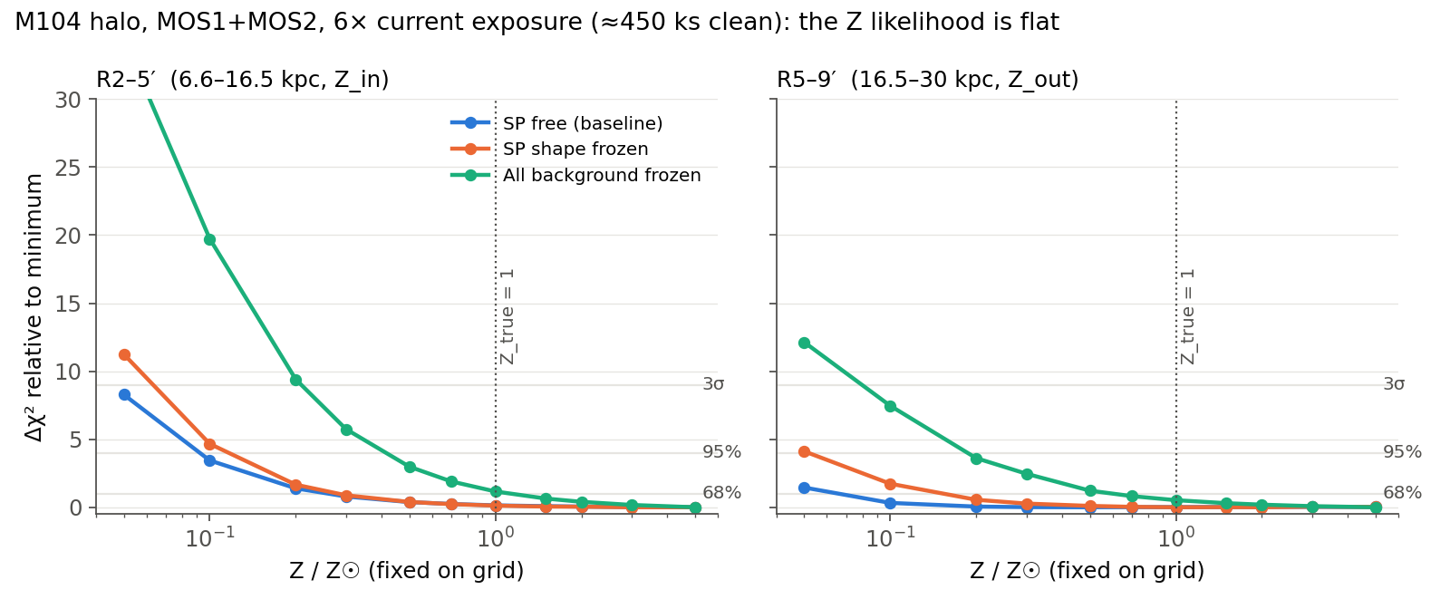
Delta chi-squared versus metallicity for the two M104 annuli under three background contracts; all curves are flat above Z of 0.3 — Figure 1. Δχ² profiles in Z for one realization at 6× the current exposure (Z_true = 1). Blue: soft-proton index and norm free (the honest contract). Orange: soft-proton shape frozen at truth, norm free. Green: all background components frozen at truth (perfect background knowledge). Horizontal lines mark 68%, 95% and 3σ.

Contract	Case	R2–5′ (Z_in)	R5–9′ (Z_out)
SP free	F = 6, Z_true = 1	Δχ² = 0.8 across 0.3–5; lower bound Z > 0.1 (Δχ² = 3.4)	Δχ² < 1.5 across 0.05–5: unconstrained
SP free	F = 6, Z_true = 0.3	Δχ² < 0.8 across 0.05–5	Δχ² < 0.5
SP free	F = 1, Z_true = 0.3	Δχ² < 4	Δχ² < 4
SP shape frozen	F = 6, Z_true = 1	Δχ² = 0.9 across 0.3–5	Δχ² < 0.3 across 0.2–5
All background frozen	F = 6, Z_true = 1	Z > 0.3 at ~2.4σ; minimum at the boundary (5); no upper bound	Z > 0.3 at ~1.6σ; no upper bound
All background frozen	F = 6, Z_true = 0.3	Z > 0.1 at ~2.7σ; no upper bound	Z < 2 at ~2σ

Even with the background known perfectly, ≈450 ks of clean MOS data give only a lower bound of 0.1–0.5 Z_☉. A Monte-Carlo grid of 8–12 realizations per configuration (F = 1, 4, 6; Z_true = 0.3, 1, 2; CXB ±10%; a 30% cool-phase injection) shows the same thing from the other side: the fitted Z clusters at the optimiser's starting values (0.3, 1.0) and at the upper boundary, Z_true = 2 is "recovered" as 1.04 ± 0.04 simply because the start was 1.0, while kT is recovered normally to ±0.02–0.06 keV. Data: summary.csv, profile CSVs.

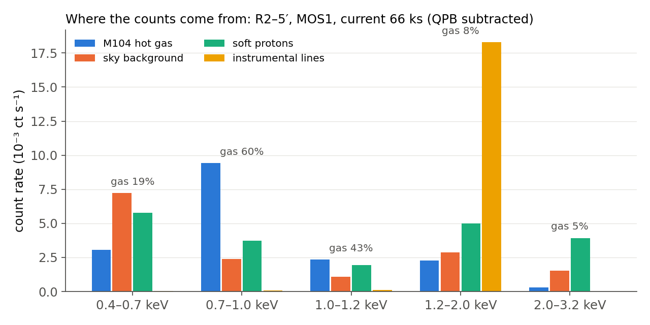
Grouped bar chart of count rates per energy band for the hot gas, sky background, soft protons and instrumental lines in the R2-5 arcminute annulus — Figure 4. Why the profile is flat. In R2–5′ (MOS1, current 66 ks) the M104 gas contributes 60% of the counts in the Fe-L band but only 8% in 1.2–2.0 keV and 5% in 2.0–3.2 keV, where the continuum that would fix Z is buried under a soft-proton power law with free index and norm and under the Al K / Si K instrumental lines. In R5–9′ the gas fraction above 1.2 keV is 2–3%. Longer exposure does not change these fractions.

Band (keV)	data − QPB	model total	M104 gas	sky	soft protons	lines	gas fraction
0.4–0.7	15.2	16.1	3.06	7.24	5.78	0.05	19%
0.7–1.0	15.2	15.6	9.42	2.40	3.73	0.07	60%
1.0–1.2	5.6	5.5	2.36	1.07	1.93	0.11	43%
1.2–2.0	28.4	28.4	2.29	2.87	4.99	18.28	8%
2.0–3.2	5.6	5.8	0.30	1.53	3.93	0.02	5%

Count rates in 10⁻³ ct s⁻¹, R2–5′, MOS1, QPB subtracted; all components in the same units.

3. Absolute metallicity: temperature × surface brightness × exposure

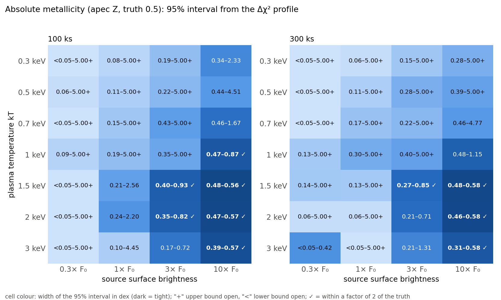
Heat maps of the 95 percent metallicity interval for seven temperatures and four surface brightness levels at 100 and 300 ks — Figure 2. 95% interval on Z (truth 0.5) from a Δχ² profile, one realization per cell, M104 background and free soft protons, 0.4–7 keV. "+" = upper bound open (profile still falling at Z = 5), "<" = lower bound open. ✓ = both bounds within a factor of 2 of the truth.

100 ks

kT	0.3× F₀	1× F₀	3× F₀	10× F₀
0.3 keV	unconstrained	0.08–5+	0.19–5+	0.34–2.33
0.5 keV	0.06–5+	0.11–5+	0.22–5+	0.44–4.5
0.7 keV	unconstrained	0.15–5+	0.43–5+	0.46–1.67
1.0 keV	0.09–5+	0.19–5+	0.35–5+	0.47–0.87
1.5 keV	unconstrained	0.21–2.56	0.40–0.93	0.48–0.56
2.0 keV	unconstrained	0.24–2.20	0.35–0.82	0.47–0.57
3.0 keV	unconstrained	0.10–4.45	0.17–0.72	0.39–0.57

300 ks

kT	0.3× F₀	1× F₀	3× F₀	10× F₀
0.3 keV	unconstrained	0.06–5+	0.15–5+	0.28–5+
0.5 keV	unconstrained	0.11–5+	0.28–5+	0.39–5+
0.7 keV	unconstrained	0.17–5+	0.22–5+	0.46–4.8
1.0 keV	0.13–5+	0.30–5+	0.40–5+	0.48–1.15
1.5 keV	0.14–5+	0.13–5+	0.27–0.85	0.48–0.58
2.0 keV	0.06–5+	0.06–5+	0.21–0.71	0.46–0.58
3.0 keV	<0.05–0.42	unconstrained	0.21–1.31	0.31–0.58

Green = within a factor of 2 at 95%. Source counts for reference (both cameras, 100 ks, 1× F₀): 1500–2000 in the Fe-L band for kT ≤ 1 keV, 700–850 for kT ≥ 1.5 keV; 3200–4600 in 0.4–7 keV. Full table with 68% intervals and best-fit values: summary_ccdZ.csv; per-cell profiles in data/profiles_Z/.

Reading the map

Temperature is the first-order control. For kT ≤ 0.7 keV, Z has only a lower bound unless the surface brightness reaches 10× F₀. The profile falls monotonically with Z: the fit prefers to give the continuum to the free soft-proton component and make the source pure line emission, so the minimum sits at the upper boundary.
For kT ≥ 1.5 keV the bremsstrahlung extends to 2–7 keV and Fe K appears; at 3× F₀, 100 ks is enough for a factor-of-2 constraint. kT = 1 keV is transitional and needs 10× F₀.
Exposure buys little in the background-dominated regime. 100 → 300 ks improves the signal-to-noise by √3 while 3× brightness raises the source fraction in the continuum bands by 3. Several 300 ks cells look no better than their 100 ks counterparts; a seed check (three realizations for kT = 0.7 / 3× F₀, kT = 2 / 1× F₀, kT = 2 / 3× F₀) shows this is realization scatter of roughly ±50% in the interval bounds, not a trend.
M104's inner halo sits in the (0.7 keV, 1× F₀) cell: 0.15–5+ at 100 ks and 0.17–5+ at 300 ks.

4. Line-to-line: the O/Fe ratio with vapec

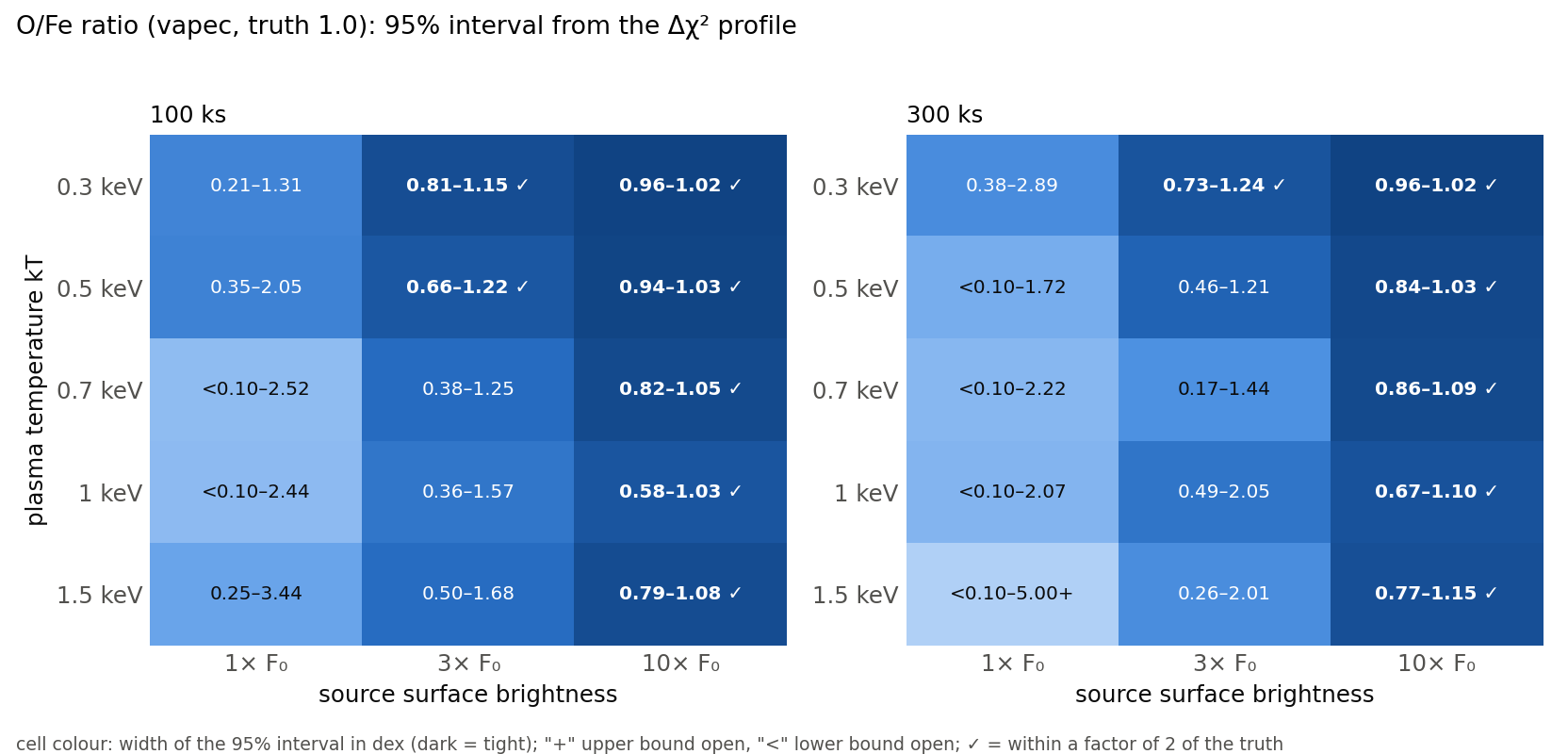
Heat maps of the 95 percent O/Fe interval for five temperatures and three surface brightness levels at 100 and 300 ks — Figure 3. 95% interval on O/Fe (truth 1.0) from a Δχ² profile with `vapec`: Fe free (Ni tied), O free (C, N, Ne, Mg, Al, Si, S, Ar, Ca tied to O), kT and norm free, soft protons and lines free. The foreground O VII / O VIII of the Local Hot Bubble and Milky Way halo are fixed at their true values (an optimistic assumption, see caveats).

100 ks

kT	1× F₀	3× F₀	10× F₀
0.3 keV	0.21–1.31	0.81–1.15	0.96–1.02
0.5 keV	0.35–2.05	0.66–1.22	0.94–1.03
0.7 keV	<0.1–2.5	0.38–1.25	0.82–1.05
1.0 keV	<0.1–2.4	0.36–1.57	0.58–1.03
1.5 keV	0.25–3.4	0.50–1.68	0.79–1.08

300 ks

kT	1× F₀	3× F₀	10× F₀
0.3 keV	0.38–2.89	0.73–1.24	0.96–1.02
0.5 keV	<0.1–1.72	0.46–1.21	0.84–1.03
0.7 keV	<0.1–2.22	0.17–1.44	0.86–1.09
1.0 keV	<0.1–2.07	0.49–2.05	0.67–1.10
1.5 keV	<0.1–5+	0.26–2.01	0.77–1.15

Source counts (both cameras, 100 ks, 1× F₀): 300–1100 in the O band (0.5–0.7 keV), 850–2040 in the Fe-L band. Full table: summary_OFe.csv; per-cell profiles in data/profiles_OFe/.

Reading the map

O/Fe is a much better CCD observable than absolute Z because both ends are lines and neither depends on the soft-proton-dominated continuum. It is constrained exactly where absolute Z fails: cool gas (kT 0.3–0.5 keV) reaches ±20–30% at 3× F₀ in 100 ks, and every kT ≤ 1.5 keV reaches ±5–20% at 10× F₀. The two maps are nearly complementary: absolute Z wants hot gas, O/Fe wants cool gas with strong O VIII.
For M104's inner halo (0.7 keV, 1× F₀) the result is still only an upper limit, O/Fe < 2.2–2.5, at 100 and 300 ks: it can exclude strongly α-enhanced gas but cannot separate a Type Ia signature (O/Fe ≈ 0.3–0.5) from solar.
M104's bulge (r < 2′, 4–10× F₀) is in the constrained region: O/Fe to ±20–30% in 100 ks, consistent with the ±0.5 obtained from 200 ks of Chandra within 5′ in the literature. The absolute Fe stays unconstrained in most cells (best-fit Fe at the boundary).

5. Caveats

MOS only. No per-annulus pn products were available. pn adds continuum counts in 1–7 keV but also background; a √2–√3 equivalent gain would shift the boundaries in Figures 2–3 by less than one brightness step and would not make the (≤0.7 keV, ≤3× F₀) cells constrained.
Foreground O lines fixed. For O/Fe the Local Hot Bubble and Milky Way halo (with their O VII / O VIII) are frozen at truth. In real data their normalisation (and solar-wind charge exchange) is uncertain at the 10–20% level and leaks directly into the source O; at 1× F₀ the source O-band counts are comparable to the foreground, so this systematic would dominate for a faint halo.
Single realization per cell. Interval bounds scatter by roughly ±30–50% between realizations (seed check in Section 3). The maps show where a constraint exists, not its precise width.
Single-temperature truth. A 30% cool-phase (0.35 keV) injection into R2–5′ fitted with one temperature biases kT to 0.53 keV and pushes Z to the start value: Fe bias and temperature bias appear together.
Statistic. chi2gehrels on subtracted, grouped data gives stat/dof ≈ 0.7 at truth; true Δχ² values are ≈1.4× larger, which does not change any conclusion.
Soft protons. The truth uses one power-law shape per camera (Γ ≈ 1.2–1.3, MOS2 norm scaled by 0.7 to match the observed rates); above 3.2 keV a single power law over-predicts the real spectrum, which only matters for the 0.4–7 keV grid fits and is consistent between truth and fit.

6. Data and code

summary_ccdZ.csv — absolute-Z grid: 68% / 95% intervals, best-fit Z, source counts, Δχ² range per cell.
summary_OFe.csv — O/Fe grid, same columns.
summary.csv — the M104 two-zone Monte-Carlo grid (recovered Z_in, Z_out, kT).
Profiles for the M104 case: SP free, F=6, Z=1, SP free, F=6, Z=0.3, SP free, F=1, Z=0.3, SP shape frozen, all background frozen, Z=1, all background frozen, Z=0.3.
Per-cell grid profiles: profiles_Z/, profiles_OFe/.
Scripts (Sherpa): fakeit_twozone_Z.py (model, fake, two-zone fit), profile_Z.py, ccd_Z_limits.py, ccd_OFe_limits.py, summarize*.py, make_figures.py.

Prepared 2026-09-24 as part of the feasibility assessment for a deep XMM-Newton observation of M104. Related published analysis of the same data: Li, Huang et al. 2026, arXiv:2609.18006.